Calculating distance is the most basic of all concepts, but it can get confusing very quickly. I hear of straight-line distance, Euclidean distance, barriers, surface distance, cost distance, vertical factor, horizontal factor, source characteristic and my head starts to spin. But all of these distance concepts tell a cohesive story that is surprisingly simple. Let me demystify it.
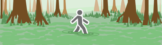
To do so I will use a single image of a hiker looking over the landscape. Put yourself in the shoes of this hiker. As you look over the landscape, there are countless decisions you can make to get from point A to point B. All of the decisions are based on how you calculate the distance between the points.

If you had wings, you could just fly over the landscape. This measure of the distance is the shortest straight-line or Euclidean distance between the two points. But if you are like me, you do not have wings.
If you start walking between the locations, there might be a lake in the way. You will need to walk around it. This diversion will increase the straight-line distance you must travel – the lake is a barrier.
As you look over the landscape you can see there are hills and mountains that you must travel over to get to the destination. To walk over the undulations, you will physically need to take more steps than if the landscape were flat. You will need to travel uphill or downhill along the hypotenuses. Thus, the increase in the number of steps will increase the distance you must travel – these additional steps determine the surface distance you must travel.
Now you have calculated the straight-line distance and adjusted it by incorporating barriers and the surface distance.
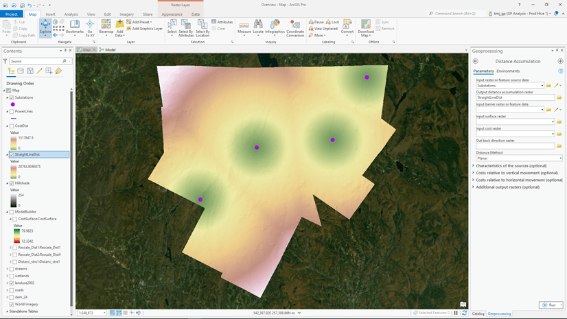
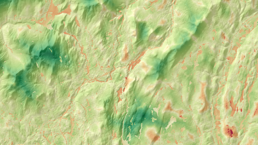
But when you look at the landscape you see forests, open fields, swamps, and various land use types. Clearly, traveling through the swamp as opposed to an open field will slow you down. These different land use types will affect the rate you encounter the adjusted distance. Determining the rate at which you can cover the adjusted distance identifies how you will experience the landscape as you move through it. You can account for this rate through a cost surface and the resulting calculations are the cost distance.
Besides the cost surface, there are three other factors that will affect the rate you will encounter the adjusted straight-line distance. Notice the mountains in the landscape. Traveling up them will require more energy and will slow you down, as opposed to traveling on flatter land. This extra effort will result in you covering the adjusted distance at a slower rate. The additional effort to overcome the slopes is the vertical factor. The vertical factor is not to be confused with the surface distance discussed above. The surface distance is the added distance you must travel moving up and down the undulations in the landscape. The vertical factor accounts for the extra effort to overcome these slopes which effects the rate you cover the distance units.
If it is a very windy day, it will be easier to move with the wind blowing from behind you than if you were traveling directly into it. This additional effort is the horizontal factor.
Instead of walking, you realize you have access to an All-Terrain Vehicle (ATV). The ATV will allow you to cover the adjusted distance units at a quicker rate. You can cover more distance at a faster rate on an ATV than if you are on foot. Your mode of travel is considered a characteristic of the source.
So where are we at? We have calculated the straight-line distance adjusting for barriers and the surface distance. We then simulated how the traveler will experience the landscape by determining the rate they will encounter the adjusted straight-line distance by incorporating a cost surface, vertical factor, horizontal factor, and source characteristics. As a result, we now know the accumulative cost to reach each location in the landscape.
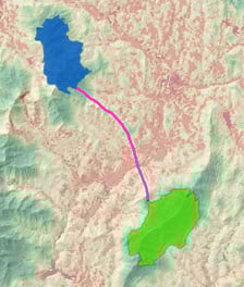
However, often we want to connect specific locations over the accumulative cost surface with optimal paths. In our example above, you know where you are starting from and you know your destination. You want to travel between the two locations by traveling the optimal path. If the cost units in our cost surface is time or effort, then the resulting path will be the path that will be the fastest or that requires the least amount of effort. To create this path, you can use the Optimal Path as Line tool.
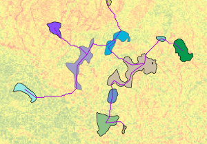
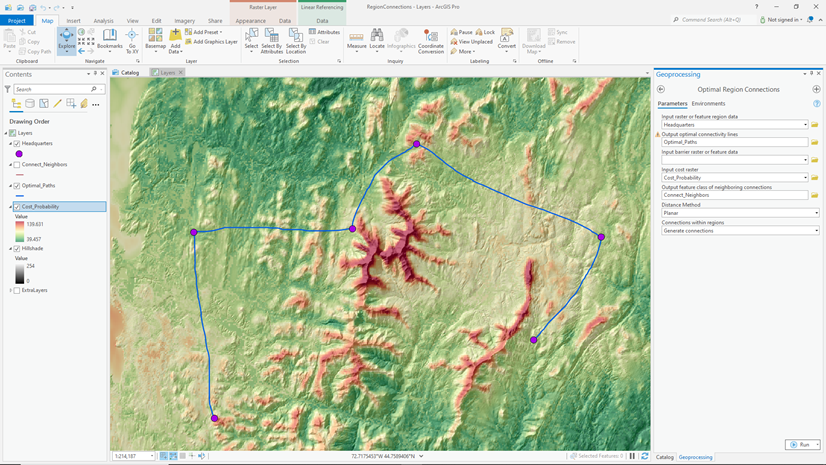
If there are a series of locations that you want to travel between, you can connect the locations with the least-cost network that will allow you to move between them. This network of paths can be created using the Optimal Region Connections tool.
As you can see, distance analysis is surprisingly simple; calculate the adjusted straight-line distance, determine the rate the adjusted distance is encountered, and then connect desired locations with optimal paths.
Even though there are many variations and modifiers that effect distance, it is all just distance.
This is the first in a series of four blogs introducing you to a new approach for understanding Distance Analysis. We have rewritten all the conceptual distance analysis documentation to make it easier for you to understand so that you can perform more effective analysis. For additional information on the conceptual framework see An Overview of Distance Analysis.
The next blog will discuss Calculating straight-line distance and adjusting it with barriers and a surface distance.
The third blog will cover determining the rate the adjusted straight-line distance is encountered through the cost surface, vertical factor, horizontal factor, and source characteristics.
The final blog will discuss three ways to connect locations with optimal connections over the cost surface through an optimal network, path, or corridor.
We hope this series of blogs will help you better understand distance analysis. The more accurately you can capture the interactions within your distance analysis, the more effective your decisions will be.

Article Discussion: