A strategy for improved locational accuracy
Editor’s note: Florida’s oldest and largest water management district developed a strategy for improving the locational accuracy of permit boundaries that have been maintained in its GIS. By using the parcel boundaries, which have a horizontal accuracy that meets or exceeds National Map Accuracy Standards, the district did not have to spend a great deal to make significant improvements in locational accuracy.
The South Florida Water Management District (SFWMD), which issues permits for consumptive water use and surface water management, needed to improve the horizontal accuracy of its permits to better support regulatory activities. About half of these permits are environmental resource permits that never expire, and the other half are consumptive water use permits that are valid for 20 years.
The permits are used by engineers, environmental scientists, hydrologists, and compliance staff to make informed decisions during the application review process and for postpermit compliance. For these reasons, it is important that even the oldest permits are depicted as accurately as possible in the GIS.
The district issued its first permit in 1972. Since that time, the GIS unit has used basemaps of varying quality to capture these features. From 1972 to 1987, permits were drawn directly on US Geological Survey 1:24,000-scale topographic quadrangle maps and Mylar overlays. From 1988 to 1995, permit boundaries were digitized using SPOT 10-meter panchromatic and 20-meter multispectral scanner imagery as the basemap. Starting in 1995, 1-meter digital orthophoto quarter-quadrangle maps were used for the same purpose.
In 1999, parcel basemaps began being used for permit locations in some—but not all—counties. Permits are correlated to parcel boundaries so parcels can be used as a control to measure the horizontal accuracy of the permits. Where a strong correlation exists between the two boundaries, parcel boundaries can replace permit boundaries. Today, all permits are digitized to the parcel level. However, the GIS contains data from previous years that is of questionable accuracy.
The Regulation Bureau of SFWMD has been using Esri products since 1991, when permits were stored in ARC/INFO coverages and edited using a menu system written in ARC Macro Language (AML). Today these permits are stored in an ArcSDE database and edited using an ArcMap extension that was written in C#. The majority of extract, translate, and load (ETL) functions, including the scripts for the Buffer-Overlay and correction phase analyses, were coded in Python.
Applying Buffer-Overlay
Positional or spatial accuracy refers to the accuracy of a test feature when compared to a control feature. Methods for determining the positional accuracy of points are well established and are usually provided as the Euclidean distance between the test point and a control point. The measure of error can be reported as errors in x, y, and z. Descriptive statistics can be generated based on these numbers.
Determining the positional accuracy of a polygon is more complicated, but there are a number of methods that can be used. The simplest to implement is the Buffer-Overlay method of Goodchild and Hunter (1997). Buffer-Overlay works by creating a buffer around a higher-accuracy control line and then noting the length of a less accurate test line within the buffer. The results are expressed as the ratio:

If the ratio is less than 1, the process is repeated with a larger buffer until the length of the test line within the buffer is greater than or equal to the control line. The accuracy of the test line can then be said to be plus or minus the buffer distance.
To thoroughly test the limits of Buffer-Overlay, a pilot area was chosen consisting of the boundaries of 259 environmental resource permits for one township/range in Lee County, Florida. Lee County was selected because it is an area known to have permits that were highly displaced from the associated parcel boundaries.
A straightforward method for determining the horizontal accuracy of the polygons that are related to parcels is to measure the offset between polygon vertices and parcel vertices and then calculate the root mean square error (RMSE). The RMSE provides a measure of accuracy for the entire feature class but does not indicate the accuracy of individual polygons, hence the need for Buffer-Overlay.
Buffer-Overlay is usually implemented by buffering a control line and quantifying how much of the test line is found within each buffer. This works well with simpler control datasets, such as shorelines, but is not practical when using parcels. In this case, there are many more control features than test features, and buffering each parcel polygon to look for a test feature is not practical.
To solve this problem, the procedure is reversed by buffering the permit lines (test) and quantifying how much of the parcel line (control) is found within each buffer. The pseudo code for calculating the initial horizontal accuracy is shown in Figure 1a.

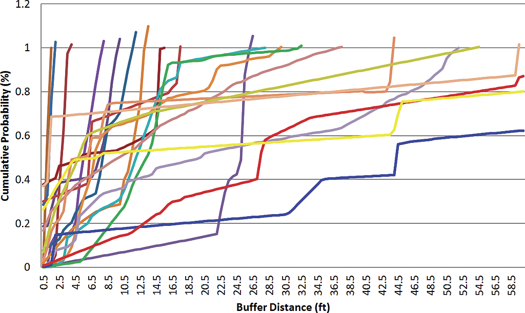
This procedure was run on all polygons in the pilot area. Figure 2 shows a random sample of the cumulative probability curves for 21 permits. On this graph, the x-axis represents the distance buffered from 0.5 to 60 feet at 0.5 ft intervals. The y-axis represents the cumulative probability. When the curve reaches 1 or more on the y-axis, the length of clipped parcel line is greater than or equal to the perimeter of the permit line. In these cases, the buffer distance is assigned as the horizontal accuracy of the permit. Those curves that never reach 1 are outside the maximum buffer distance of 60 feet.
Correction Phase
The next logical step involved building the extracted parcel line segments into polygons using the topology tools in ArcMap. In some cases, line segment artifacts are extracted that form closed rings and result in polygon builds that are significantly larger or smaller in area than the original permit. These are excluded through an area comparison. The pseudo code for the correction is as follows:
The confidence interval on the estimate of RMSE for x and y at 95 percent probability was calculated using 30 coordinate pairs from the pilot area at the initial condition and after correction (shown in Table 1). The RMSE measures are circular for both conditions. This means that the values are relatively similar between x and y and indicate that there is no systematic error in the data that would produce more errors in any particular direction. After Buffer-Overlay, the corrected RMSE x values dropped by 4.7 feet from 20.22 ± 5.74 to 15.52 ± 5.78. Corrected RMSEy values dropped by 9.42 feet from 22.18 ± 7.29 to 12.76 ± 4.6. This indicated a significant improvement in the data.
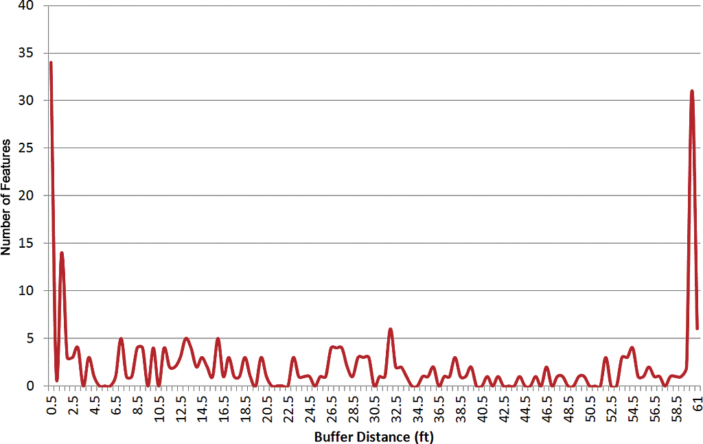
A graph of the initial horizontal accuracy distribution from 0 to 60 feet for all 259 permits shows two peaks at either extreme. On the left side of the graph, 13 percent of the data (or 34 features) had high accuracy, with horizontal displacements from parcels of 0.5 feet. On the right side of the graph, 12 percent of the data (or 31 features) had low accuracy, with horizontal displacements from parcels of 60 feet. Between these two peaks, the curve was skewed to the left but otherwise randomly distributed and contained 75 percent of the data (Figure 3).
The Correction Phase involved replacing the permit boundaries with the polygons built from the clipped parcel lines. Once this was complete, RMSE for the feature class was recalculated (see Table 1) and Buffer-Overlay accuracies for each of the 259 permits were recalculated.

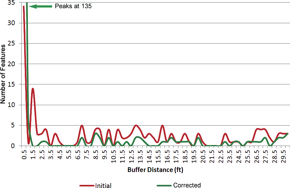
The graph in Figure 4 shows the initial (red) and corrected (green) distributions for permit boundaries with accuracies between 0 and 30. After correction, 52 percent (135 features) of the data had high accuracy of 0.5 feet. Note that the corrected curve runs above the initial curve for accuracies of 1 foot. The percentage of records between 0.5 and 60 feet was reduced from 75 percent to 40 percent. Notice that the amplitude of the corrected curve (green) was reduced and runs below the initial curve for buffer distances from 1 to 60 (as expected). Finally, 12 percent of the data still had low accuracy (i.e., > 60 feet) representing features with accuracies beyond the 60-foot maximum buffer distance.
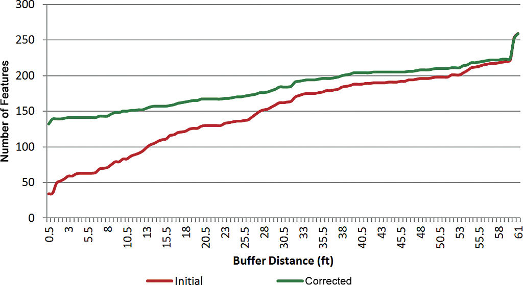
The graph in Figure 5 shows the cumulative horizontal accuracy distributions. In the best-case scenario, this would be a straight line across the y-axis at 259 indicating that all features had accuracies of 0.5 feet. The red curve represents the initial conditions, with 13 percent of features having accuracies of 0.5 feet; the green curve represents the correction with 52 percent of features having accuracies of 0.5 feet.
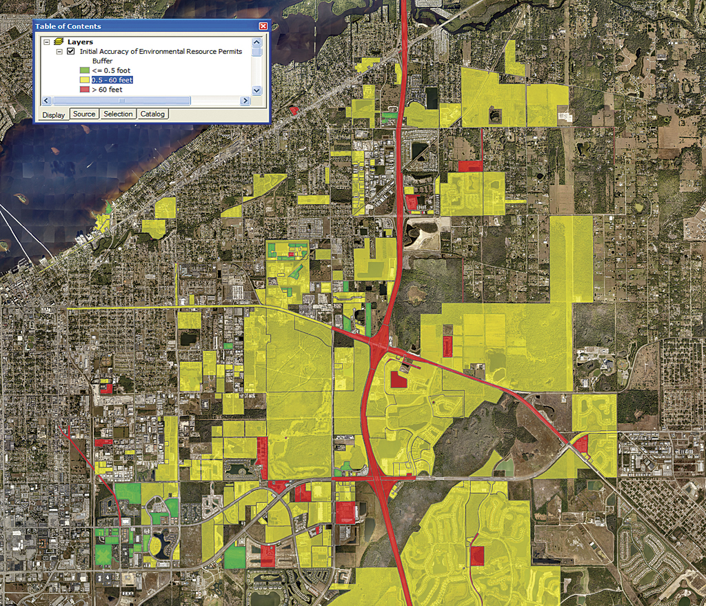
The two maps in Figures 6a and 6b below depict the horizontal accuracy at the initial condition and after correction. Green boundaries have accuracies of 0.5 feet, yellow boundaries have accuracies from 0.5 to 60 feet, and red boundaries have accuracies > 60 feet. The second map shows a significant increase in the number of permits with accuracies of 0.5 feet.
Conclusion
Most data stewards would acknowledge they have data that should be improved but lack the time and money to make improvements. Many of these datasets are based on or directly related to higher-accuracy datasets that could be used as controls to determine and improve horizontal accuracy.

In this example, Buffer-Overlay was used to determine and improve the horizontal accuracy of environmental resource permits using parcels as controls with excellent results. Buffer-Overlay is conceptually simple. It uses buffer and clip, two of the most common geospatial operators, and is easy to automate. The cost of improving data using Buffer-Overlay is low, confined to algorithm development and CPU cycles, leaving the data steward free to focus on other more important tasks.
References
Goodchild, F. M., and G. J. Hunter, 1997. “A Simple Positional Accuracy Measure for Linear Features,” International Journal of Geographical Information Sciences, 11(3):299–306.
About the author