Defining and managing a local grid in ArcGIS 10.1
This article builds on the techniques learned in “Good, Better, and Best: Converting and Managing Local Coordinates in a Projected System,” which ran in the Spring 2013 issue of ArcUser magazine.
That exercise showed how to place a locally referenced scanned map and a computer-aided drafting/design (CAD) drawing in a projected coordinate system. Using the ArcGIS 10.1 Georeferencing tool, local control points were connected to coordinates that were surveyed in the field. By connecting a high-quality scanned map and CAD layer to carefully surveyed points, both products were georeferenced with surprising precision.
Continuing to Battle the Mountain, Locally
Like the previous exercises, this exercise uses data related to mining activity around the Old Rattler claim in Battle Mountain, Nevada. The data includes completely synthetic drill hole collar locations and topographic survey control data for more than 80 holes drilled in 1978 and 1979. In the previous exercise, we inspected the relative locations of many drill hole collars that were originally defined in a local grid, changed the scale and units, and compensated for a rotated local grid.
Unfortunately, due to the quality of the scanned map and limitations of the CAD file, we could not validate the data. However, during a subsequent search of legacy data, we discovered an old database file containing information about 84 exploration holes drilled in 1978 and 1979. The simple collar file includes drill hole names, local coordinates, total depth, and orientation. The file also includes local coordinates for survey points labeled Control 1 through Control 4. It would be great if these collar points were registered in Universal Transverse Mercator (UTM) North American Datum (NAD83), but this is enough information to get started moving them to projected coordinate space.
DHA-78-001 marks the origin of the local system, so we sent the surveyors back to the field to precisely capture its coordinates in UTM meters and NAD83 decimal degrees. The major axes of the local grid are rotated about 17 degrees to the right (clockwise), which approximates the local magnetic north in the late 1970s. Since we are not sure field staff who collected the original data even understood datums, we will register the local grid in NAD83. All early field measurements seem to be recorded in feet, so we will specify US Survey Feet as the local unit.
First, we will need to create a new data frame in the existing project, then post the collar points, add the known UTM NAD83 Survey Control as a reference, and experiment with local grid parameters to see if we can match local control with a known survey. This might sound quite complicated, but the matching process is very hands-on and visual, though it often requires multiple iterations to define the best fit.
Legacy Data on Drill Hole Collars
Download the sample dataset [ZIP] and unzip it locally.
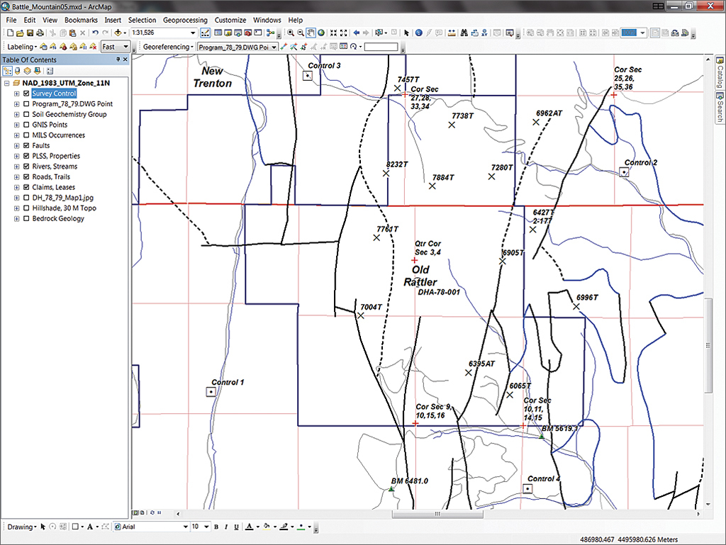
- Open Battle Mountain05.mxd in ArcMap. Zoom to the extent of Survey Control layer and make only the Survey Control, Faults, PLSS, Properties, Rivers, Streams, Roads, Trails, Claims, and Leases layers visible. Save the project, renaming it Battle_Mountain06.
- To begin, insert a new unprojected data frame. On the Standard menu, choose Insert > Data frame. Do not add any data because ArcMap will adopt the projection used by that data. Right-click New Data Frame and choose Properties.
- In the General Tab, rename the data frame Local Grid, set the Map Units and Display Units to Feet, and activate the Maplex Label Engine. Click the Coordinate System tab and verify that no coordinate system is specified. Apply these updates and save the project. Local Grid is now the active data frame.
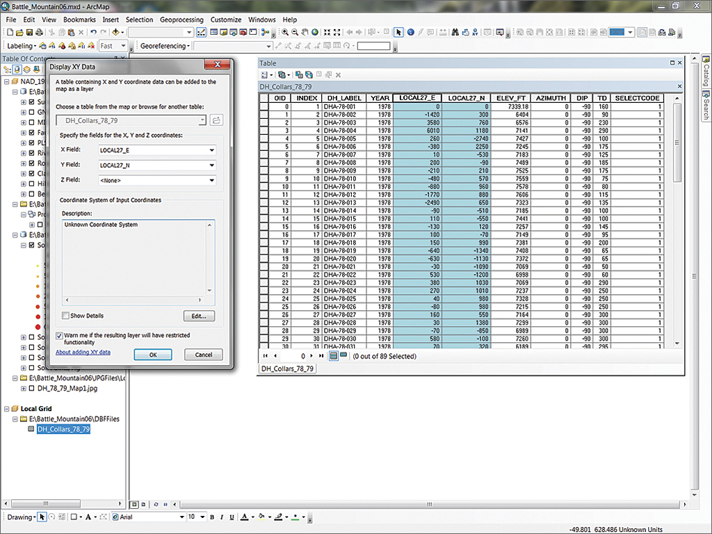
- Click the Add data button, navigate to \Battle_Mountain05\DBFFiles, and load DH_Collars_78_79.dbf. Inspect this table of legacy data and observe the local Easting (LOCAL27_E) and Northing (LOCAL27_N) fields. Someone made a very general assumption that the datum might be NAD27 (if a datum was even considered). Scroll to the bottom of the table to see the four control points used in the previous exercise.
- In the table of contents (TOC), right-click DH_Collars_78_97.dbf and select Display XY Data.
Set X Field: to [LOCAL27_E] and Y Field: to [LOCAL27_N].
Leave Z Field: set to , as we have not validated [ELEV_FT].
DO NOT define a Coordinate System.
Click OK. - Change the point symbol to something distinctive such as the red 14-point crosshair symbol. Check the coordinates of the four bounding control points. These points no longer have the units of measure assigned to them previously and have reset to Unknown Units. Reopen the data frame properties and change units back to Feet.
- Bring the Survey Control reference data into the new data frame. Change the TOC display to List by Drawing Order and make the NAD_1983_UTM_Zone_11N data frame the active data frame. Right-click Survey Control and choose Copy. Right-click the Local Grid data frame name and select Paste Layers(s). Position the Survey Control layer below DH_Collars_78_79 Events and expand its legend. The UTM NAD83 survey data provides a reference that can be used to determine the projection parameters for the local system data. Save the project again.
Chasing the Rattler: The Fun Starts
This is the challenging part of our adventure. The well-defined UTM NAD83 survey data has been added to the Local Grid data frame which also contains the mapped origin and widely spaced control points of the local grid. The grid origin (we think) was aligned using magnetic north, and map units are certainly imperial (feet).
The grid origin is essential. Our surveyors just returned from the field with very carefully derived longitude and latitude in World Geodetic System 1984 (WGS84) for the collar of DHA-78-001. This information should be sufficient to define a coordinate system for the Local Grid data frame. Once it is created and tested, this local coordinate system can be saved to the Favorites in the list of ArcMap’s projections so it can be used to register other early project data including the Program_78_79 CAD drawing.
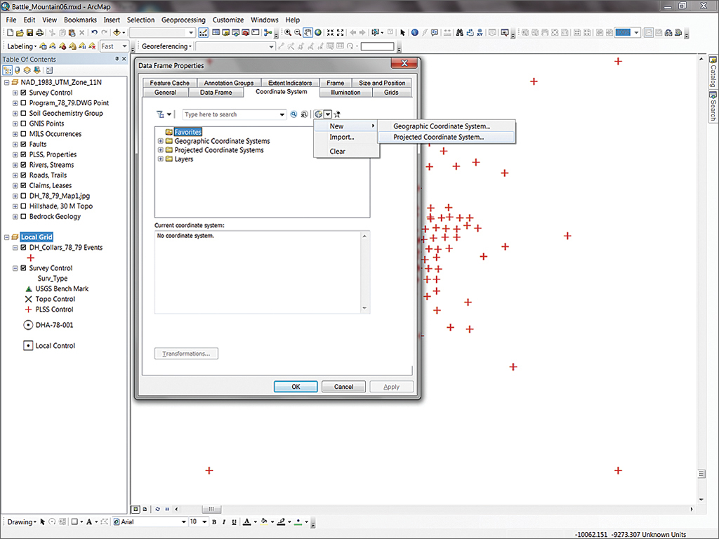
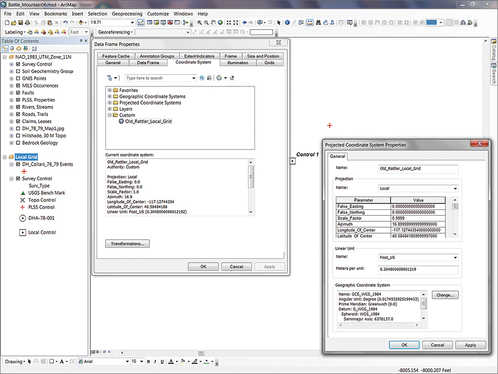
1. Open Properties for the Local Grid data frame and select the Coordinate System tab. Mouse over the small icons to the right of the search window to locate the Add Coordinate System icon and click its drop-down arrow.
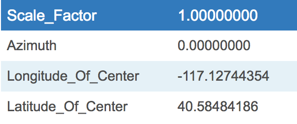
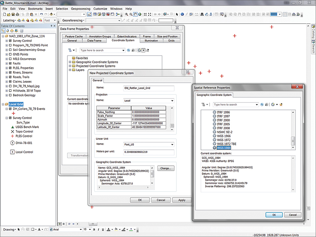
2. Choose New > Projected Coordinate System. Name the new coordinate system Old_Rattler_Local_Grid. Change the Projection Name to Local. Now fill in some of the blanks. Scroll down past False_Easting and False_Northing and type in the values in Table 1 for some other parameters. Our surveyors collected very precise WGS84 geographic coordinates for the origin drill hole, DHA-78-001. Longitude and latitude values are necessarily very precise, representing centimeter-level measurements. Check them carefully as you enter these values.
3. Set Linear Unit to Foot_US and change the Geographic Coordinate System to GCS_WGS_1984. Click OK twice to update the Local Grid coordinate system.
4. The Tranformations warning box appears. Click Yes (Remember, never check the box next to Don’t warn me again ever). Click OK twice.
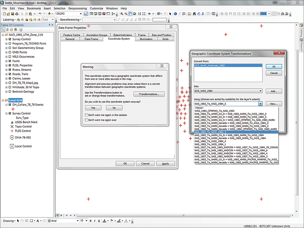
5. Return to the Coordinate tab and click the Transformations button. In the Geographic Coordinate Systems Tranformation dialog box, set Convert from: to GCS_North_American_1983; set Into: as CGS_WGS_1984, and set Using: to NAD_1983_To_WGS_1984_5. This is a very important step. Click OK to close Data Frame Properties and apply the update.
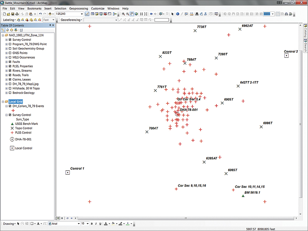
6. Zoom to the layer extent and see how well the control points on the drill collars data matches Survey Control points. Zoom to the DHA-78-001 (the origin that is labeled) and check its coordinates. They should be very close to (but perhaps not exactly) 0,0. If you have a difference of more than a foot, return to the data frame’s Coordinate System properties and check the values entered for the longitude and latitude center coordinates. Save the project.
7. Notice that four red crosshairs in the display’s corners are still orthogonal (i.e., not rotated). This will be fixed interactively in a later step. Zoom back to the extent of the Survey Control layer and save the project. With the origin pinned, we are on our way to defining a local coordinate system.
Modifying Our Local System
After defining the origin, we can focus on the grid’s rotated azimuth.
- Reopen the Local Grid Properties and click the Coordinate System tab. Double-click Old_Rattler_Local_Grid and set the Azimuth: to 17 and click Apply.
This rotation approximates the magnetic declination in northern Nevada in 1978. If your local grid has an unknown rotation, you can calculate it geometrically from known points in local and projected systems or just experiment. If your local grid applies False Easting and False Northing offsets (some do to avoid negative coordinate values), find out what they are and include them, expressed in local units.
- Now see if survey and drill collar data control points are coincident. Zoomed out, they should appear very close. Zoom in to Control 2 and measure the distance between Control 2 and its companion point in the collar table. The collar control point should appear to be about 20 feet southeast of Control 2. Remember that the grid rotation was set to 17 degrees, which appears to be too far. Do not change the view scale.
- Return to Coordinate System properties and set Azimuth to 16.8. Apply the change and study the difference. Now the collar control point falls about 20 feet northwest of Control 2. Split the difference and try an azimuth of 16.9 degrees. Reset the azimuth and check the results. This time, zoom way in to Control 1 and measure. The collar control should be only a foot or so from Control 1. Notice that the collar point is directly northeast of Control 1, located southwest of the grid’s origin. Let’s fine-tune our coordinate system next. Save the project.
Tuning and Saving Our Local Grid
Remember the Scale_Factor parameter? It might be the least understood of all projection parameters, but it is very important. A very slight stretch to the local system is needed to obtain a best fit. Return again to Coordinate System properties, set a Scale_Factor of 0.9999, apply the change, and zoom way in to Control 1 to inspect the results. Check out the DHA-78-001 origin and the other three control points. The differences between control points and collar points should be very small. Tweaking the origin would get them a bit closer; but controls points are already well within the tolerances that our surveyors might achieve. Save the project again to preserve the Local Grid settings.
Now save this local coordinate system so it can be applied to other spatial datasets, including CAD data. This acceptable local grid can be saved to our Favorites in ArcMap. Open Coordinate System properties and observe the rightmost, star-shaped icon. Highlight Old_Rattler_Local_Grid and click this button to save this coordinate system to your Favorites. The Old Rattler coordinate system will now be available whenever needed.
Managing the Local Grid
All or some of the DH_Collars_78_79 Event points can be exported as a shapefile or a feature class.
1. Right-click the DH_Collars_78_79 Events layer in the Local Grid data frame and choose Data > Export Data. Save the shapefile in \SHPFiles\Local as DH_Collars_78_79 and click Yes when asked if you want to add this layer to the project and use the coordinate system of the data frame. Change the symbol to a green X and zoom to the map extent. Now for the real test.
2. Copy the DH_Collars_78_79 shapefile layer in Local Grid and paste it into the NAD_1983_UTM_Zone_11N data frame. Make the NAD_1983_UTM_11N data frame active and zoom to the extent of the DH_Collars_78_79 layer. Carefully study the map. Notice the properly rotated control points match the origin drill holes. Save the project.
3. Before applying the Old Rattler coordinate system to the Program_78_79.DWG Point data, a little “housecleaning” is needed. The two-point CAD world file previously used to register the Program_78_79.DWG Point file should be removed from the project and any reference to this earlier relationship erased. The best way to do this is to first remove Program_78_79.DWG Point from the UTM data frame, save the project, and close ArcMap.
4. Open Windows Explorer or another file manager and navigate to \Battle_Mountain06\CADFiles\Local and delete all files under Program_78_79.DWG except Program_78_79.DWG.Points (including the .lyr, .xml, and especially the .wld files).
5. Restart ArcMap and reopen the project. In ArcMap, open the ArcCatalog window, navigate to \CADFiles\Local, and locate Program_78_79.DWG.Points. Right-click the CAD file and select properties. Open the General tab and notice that the Spatial Reference is undefined. Click the Edit button and select Old_Rattler_Local Grid from Favorites. Click OK several times to assign this coordinate system. Open Properties for Program_78_79.DWG Points to verify that the coordinate system has been applied.
6. To test this CAD projection, drag just Program_78_79.DWG Points to the ArcMap canvas. These points should post right on top of the DH_Collars_78_79 points. In the background, you created a standard Esri projection file that is located in the same folder. It has the same root name as the CAD drawing and a .prj extension.
Tip: Want to know how ArcMap stores the information about coordinate systems you save as Favorites? In ArcCatalog, browse to C:\Users\<your user name>\AppData\Roaming\Esri\Desktop10.1\ArcMap\Coordinate Systems.

Summary
This tutorial actually uses the same steps covered in the previous article “Good, Better, and Best: Converting and Managing Local Coordinates in a Projected System,” in the Spring 2013 issue of ArcUser magazine, but this time these steps were performed in a different order to define a local coordinate system in a new data frame.
- Move: Use geographic coordinates to define the local origin.
- Rotate: Experiment with the local azimuth to align survey control.
- Scale: Use adjusted US Feet units to minimize distortion away from the local origin.
In this tutorial, we won the fight with Battle Mountain by successfully defining a local coordinate system that will properly register local vector data in any data frame containing a properly defined coordinate system.

Try this three-step approach with other local data. Remember that you must obtain the highest-quality survey data available to define a local origin and any Easting/Northing offset. Also, you must calculate (or carefully estimate) any grid rotation. Always reinspect the data as you tune the coordinate system. Feel free to contact me and let me know how this method works for you.
Acknowledgments
Thanks again to the US Geological Survey (USGS), the Geological Survey of Canada (GSC) and Geoscience Australia (formerly Australia Geological Survey Organisation that have developed the basemap data that support this training series. And special thanks to my geologist and firefighter friends who support and test these tutorials. I could not create field-ready materials without their valuable input and assistance.