This article discusses multivariate interpolation using cokriging methods and how the cross-covariance graphs produced using the ArcGIS Geostatistical Analyst extension can model variables’ spatial dependence. It also describes how data from a petroleum study was analyzed using multivariate interpolation with cokriging methods to select optimal additional well locations for the study area.
In many applications, including environmental monitoring, atmospheric modeling, real estate markets, and forestry, several spatially dependent variables are recorded across the region. The multivariate spatial interpolation model (called cokriging) requires specification of valid and optimal correlation and cross-correlation functions. Using these functions, cokriging combines spatial data on several variables to make a single map of one of the variables using information about the spatial correlation of the variable of interest and cross correlations between it and other variables.
This article discusses cokriging methodology and illustrates its usage with real oil and gas data collected in several hundred wells. A series of probability maps were created showing well performance index using kriging models and also using cokriging with permeability of the rock, depth to top of shale (which would affect the pressure at which the gas is produced), and total clean volume pumped (i.e., the amount of liquid pushed into the well) as secondary variables. The proper use of these additional variables significantly improves spatial predictions that are used for future gas and oil production planning.
Understanding Multivariate Interpolation
The prediction of multivariate spatial processes is an important problem in many research areas in geology, environmental monitoring, meteorology, real estate markets, and agriculture. Because they are expensive to collect, in many cases only a limited number of data points are available.
Consequently, it is desirable that all available observations be taken into account. Their contributions should be weighted by the strength of their correlation with prediction locations. A typical example is mapping air pollution. Predictions can be improved by using distance from roads and measurements of other pollutants. Multivariate interpolation modeling, today known as cokriging, was first used to improve prediction of the earth’s gravitational field using data from wind measurements made by Lev Gandin in 1963.
Cokriging models are efficient, but they require certain restricting assumptions, in particular, assumptions about data normality and stationarity. These assumptions are often unrealistic, but they serve as building blocks for more sophisticated models.
In the ArcGIS Geostatistical Analyst extension, one, two, or three variables can be used as secondary variables for making more accurate predictions of the primary variable at the unsampled location. The prediction is a weighted sum of the observations in the searching neighborhood.
Applying Cokriging
For the examples shown in this article, a dataset containing production data from 381 wells collected between the beginning of 2009 and the end of 2010 was used. This data is owned by Chesapeake Energy Corporation and was used with permission on the condition that no locational information be disclosed.
In Figure 1a, the prediction at the shovel location is a weighted sum of three measurements of the variable Z. Coefficients a1, a2, and a3 are functions of the covariance model, which describes the spatial correlation of Z. In Figure 1b, the prediction at the shovel location is a weighted sum of three measurements of the variable Z and two measurements of the variable X. Coefficients b1 and b2 are functions of the cross-covariance model, which describes spatial correlation between Z and X. Therefore, the secondary variable X is used as an additional set of the measurements.
Figures 2a and 2b show cross-covariance models (blue lines) with positive (Figure 2a) and negative correlation (Figure 2b) between two variables. Crosses and red points show cross-covariance values averaged at particular intervals of distances between pairs of points and angles.
If variables are spatially independent, cross-covariance is equal to zero. The weights of the secondary variables are also zero. The predictions using kriging and cokriging are identical, as the secondary variables are ignored.
If cross-correlation exists and is estimated correctly, cokriging outperforms kriging simply because it is based on a larger amount of information. However, the prediction quality may decrease if cokriging model parameters are estimated incorrectly.
To summarize, all that is required for optimal multivariate prediction is an accurate estimation of several correlation functions. This can be done interactively using the Geostatistical Wizard in the Geostatistical Analyst extension.
Evaluating Oil and Gas Data
Several factors go into deciding whether to drill a well. A primary factor is how much petroleum a well can be expected to produce. A sound economic decision will be based on the expected return on investment. With the data examined in this example, the goal is to find areas that will produce the most petroleum. Once those areas are determined, a separate economic analysis would be required to determine how much profit could be generated from each well. In evaluating the profitability of the wells in this example, $97.98 per barrel for oil and $3.73 per Mcf. [1,000 cubic feet] for gas were used.
A well performance index (WPI) was used to estimate how productive a well would be. WPI is the daily rate at which petroleum is produced multiplied by the daily pressure, summed over the first 90 days of production. This was the main variable that was interpolated to help decide where to drill for the most productive wells. WPI values range from 45,000 to 750,000, so a quick economic analysis determined that the minimum WPI at which a well would become profitable was 250,000. Although a well could exceed this WPI and be unprofitable, areas below this performance threshold would not be of interest.
For every oil and gas well drilled, several geophysical and operational parameters are measured during the drilling process. Over time, this information paints a picture of the spatially dynamic characteristics of the petroleum reservoir under extraction. After reviewing these parameters, the list of parameters was limited to the ones that were expected to have the biggest impact.
The secondary variables expected to influence the WPI are permeability of the shale rock, the depth to the top of the shale formation, and the total clean volume pumped into the well during the fracking process.
Permeability measures how easily oil and gas can flow through rock. The higher the permeability, the easier it is for petroleum to leave the rock through fractures (both natural and man-made) and enter the wellbore. Therefore, the general assumption is that higher permeability will correlate with a higher WPI.
The depth to shale rock is dynamic and can change several hundred feet across a reservoir and dramatically at fault lines. One of the impacts this measurement has on oil and gas production is as an indicator of the amount of pressure the rock is under. The deeper the rock occurs, the higher the pressure, and vice versa. Therefore, the assumption is that a higher pressure well will produce more oil and gas more quickly than a lower pressure well.
The final variable, total clean volume pumped, is an operations-side consideration. It is a measurement of the amount of liquid pumped into the wellbore to create man-made fractures in the shale rock. Once again, the assumption is that bigger is better. The higher the volume pumped, the larger and more numerous the fractures created, allowing more oil and gas to flow into the wellbore and positively impact WPI.
The Effect of Incorporating Secondary Variables
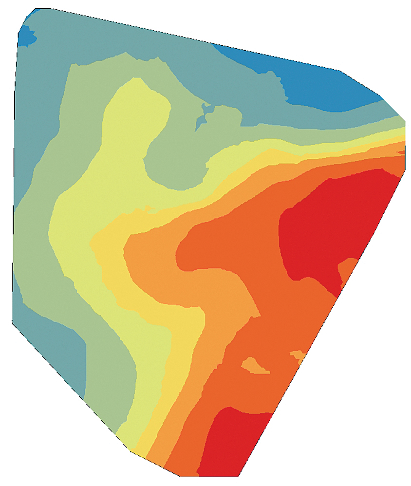
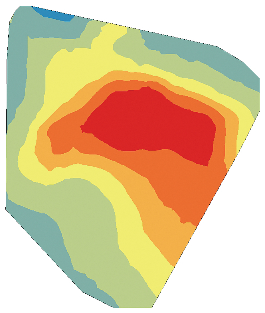
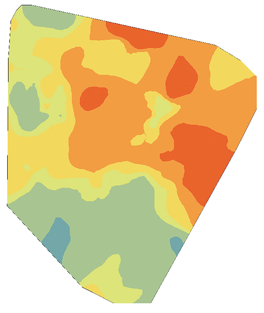
The cokriging output surface, especially when the secondary variables are sampled more densely than the primary variable, produces a more realistic depiction of the data by extracting additional information from the secondary variables. Figures 3a, 3b, and 3c are interpolated maps of the three secondary variables (the depth of the top of the shale formation, permeability of the shale rock, and the total clean volume pumped). Figure 3d shows the cokriging WPI prediction, which extracts information from both primary and secondary variables through their correlation functions.
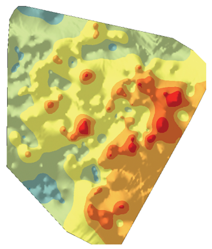

New well sample locations for drilling can be selected using a spatially balanced design algorithm that was discussed in “Unequal Probability-Based Spatial Sampling,” an article by Konstantin Krivoruchko and Kevin Butler that appeared in the Spring 2013 issue of ArcUser. This design algorithm uses the inclusion probability raster, which defines an a priori sample intensity. The inclusion probabilities can reflect both statistical data features, such as kriging predictions and prediction standard errors, and all relevant geologic information and the reservoir engineers’ expert knowledge. Each raster cell with nonzero inclusion probability has a chance of being selected. Figure 4 is an inclusion probability map showing areas in red and warm colors where wells might be profitably added. Gray circles show 10 optimal candidate locations for drilling.
Further Reading
Krivoruchko, Konstantin. Spatial Statistical Data Analysis for GIS Users. Esri Press, 2011, 928 pp.
Krivoruchko, Konstantin, and Kevin Butler. “Unequal Probability-Based Spatial Sampling,” ArcUser Spring 2013, pp. 10–17.
For more information, contact Nathan A. Wood.
About the authors