ArcUser
Winter 2012 Edition
More Emergency Services Modeling
Analyzing changes in response using Network Analyst
By Mike Price, Entrada/San Juan, Inc.
This article as a PDF.
Sample dataset
 This tutorial shows how to use the Closest Facility (CF) solver in ArcGIS Network Analyst to model travel from a single facility to the closest incidents. The model will be modified to reflect proposed changes in station locations.
In the current economic climate, public safety administrators and planners are often faced with complex decisions regarding moving or closing essential facilities. Fire station closure, consolidation, or relocation studies occur throughout the United States. Public safety officials try to make best use of existing resources and provide comparable or improved levels of service. To analyze existing and future conditions, comprehensive data is required to represent current conditions, reflect past performance, and plan for the future.
To begin the exercise, open Redlands_Fire01.mxd in ArcMap.
In Esri's home town of Redlands, California, the Redlands Fire Department is facing considerable commercial and residential growth in the northern part of the city. Redlands is currently protected by four fire stations in Redlands and a station in Loma Linda, located to the west.
In 2010, Redlands firefighters and emergency medical technicians (EMTs) responded to more than 8,000 incidents in and around the city. By mapping the likelihood of where, when, and how incidents have occurred, historic incidents often provide the best estimate of community risk. Historic risk is used to demonstrate an adequate Standard of Coverage; identify underserved, problem, or frequent call locations; and project future demand for services.
The CF solver in ArcGIS Network Analyst is an excellent tool for modeling optimal travel from fixed facilities to historic incidents. By adding or substituting new or relocated stations in CF templates, it is easy to perform multiple analyses.
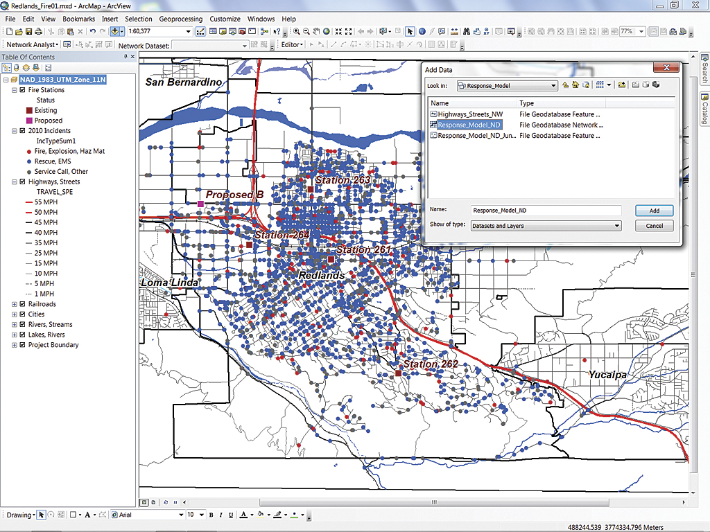
In the Fire Data geodatabase, expand the Response_Model feature dataset and add only the prebuilt Response_Model_ND network dataset.
Getting Started
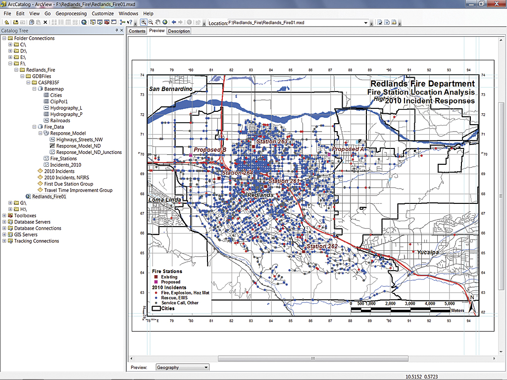
To begin this exercise, download the zipped training dataset. Unzip it in a project area on your computer. Open ArcCatalog and navigate to the \Redlands_Fire folder and explore its contents. This project contains two file geodatabases and several small utility files. The training data is projected in California State Plane North American Datum 1983 (NAD83) Zone 5 US Feet. To support a US National Grid spatial reference, the data frame projection is set to universal transverse Mercator (UTM) NAD83 Zone 11 Meters.
Inspect the geodatabase feature classes and layer files in the geodatabases. In the Fire Data geodatabase, open the Response_Model feature dataset and inspect Response_Model_ND. To quickly start the analysis portion of this tutorial, a very functional network dataset was prebuilt.
Notice that two layer files, First Due Station Group and Travel Time Improvement Group, cannot be viewed. Do not load them until instructed. These layer templates will be added to the map later to display results.

To load incidents, right-click Incidents and click Load From 2010 Incidents. Set the Sort Field to OBJECT_ID and select Inc_Number for Name. Click OK and wait patiently as all 8,173 incidents load.
Modeling Response with Network Analyst Closest Facility Solver
The CF solver is traditionally used to locate one or more destination facilities within reasonable travel time of a specific incident. Turned upside down, the CF solver maps travel from one or more fixed facilities to multiple incidents. In this exercise, the CF solver will be used to model travel away from single facilities toward the closest incidents, but facilities will be modified to reflect station changes.
Using actual 2010 incidents and a section clipped from the street network provided by the regional dispatch center, this tutorial will use the CF solver to compare optimal existing coverage to coverage provided by adding one or two proposed stations in northern areas of Redlands. For another innovative use of the CF solver, see another article in ArcUser, "Run Orders: Modeling and mapping public safety arrival orders," in the Fall 2009 issue.
- To begin the exercise, close ArcCatalog and start ArcMap. Open Redlands_Fire01.mxd and inspect its contents. If you completed the exercise in the article "Analyzing Frequent Response: Using a US National Grid spatial index" in the Summer 2011 issue of ArcUser, this map will look very familiar.
- Open and inspect the 2010 Incidents attribute table. Study the rightmost fields that are filled with zeros. These fields will be used to record response statistics. The table includes fields for station numbers and travel times to accommodate a base case and three scenarios. Three fields on the far right will soon contain differential travel times between the base case and each scenario. This map includes a new time-based street dataset so its network dataset must now be loaded.
- Switch from layout to data view. Click Add Data and navigate to \Fire_Data\. Expand the Response_Model feature dataset and add only the Response_Model_ND file geodatabase network dataset. Do not add other participating feature classes.
- In the table of contents (TOC), move Response_Model_ND below Highways, Streets and make it nonvisible. If necessary, enable the Network Analyst extension and load its toolbar.
- Save the project.
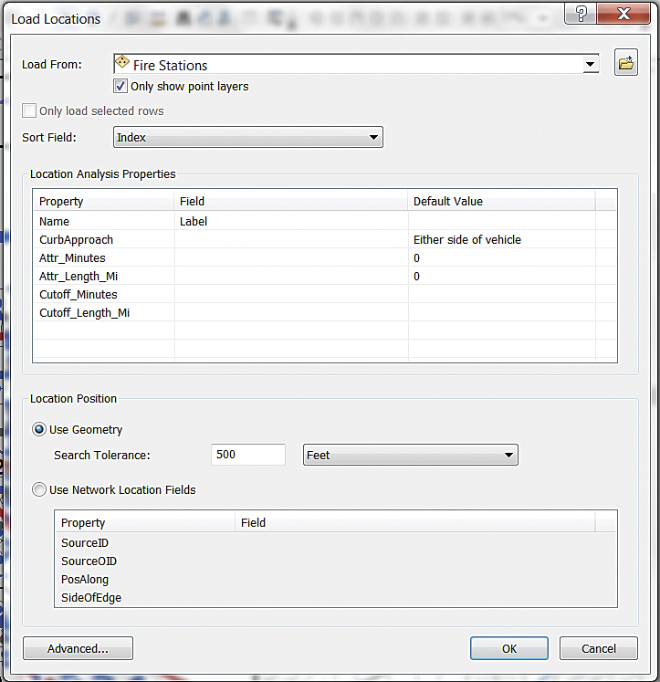
Right-click Facilities and select Load Locations. Set Load From to Fire Stations, Sort Field to Index, Name to Label, and Search Tolerance to 500 Feet and click OK.
Creating a Closest Facilities Template
- In the Network Analyst drop-down, select and load New Closest Facility.
- Once loaded, open its properties and click the Analysis Settings tab. Set Travel From to Facility to Incident and Facilities to Find to 1. Under the Accumulation tab, check both Length_Mi and Minutes. Click the General tab and name the solver Redlands CF Template.
- Before cloning this template, all facilities and incidents will be added using the Network Analyst window. From the Network Analyst toolbar, click the Network Analyst Window button and dock the window to the right of the TOC.
- Right-click Facilities and select Load Locations. Set Load From to Fire Stations, Sort Field to Index, Name to Label, and Search Tolerance to 500 Feet. Click OK and check your work.
- To load incidents, right-click Incidents and click Load From 2010 Incidents. Set the Sort Field to OBJECT_ID and select Inc_Number for Name. Click OK and wait patiently as all 8,173 incidents load.
- Choose the bookmark Redlands Fire 1:60,000 and verify your work.
- In the TOC, right-click the Redlands CF Template and select Copy. Right-click the data frame name and select Paste Layer(s). Repeat this procedure until you have four copies of the original Redlands CF Template at or near the top of the TOC.
- Select all five Redlands CF Template layers and right-click any one of them. Choose Select Group, rename the Group layer Redlands CF Group, make all group elements nonvisible, and move the group to the bottom of the TOC.
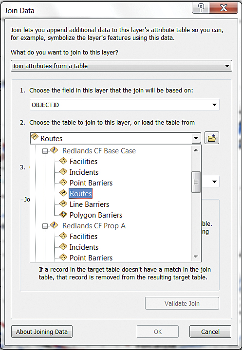
In the TOC, right-click 2010 Incidents and choose Joins and Relates > Join. For Item 1, select OBJECTID, and for Item 2, specify Redlands CF Base Case > Routes. Be sure to specify Base Case!
Building and Solving Multiple Scenarios
- Rename the first four CF templates as Redlands CF Base Case, Redlands CF Prop A, Redlands CF Prop B, Redlands CF Prop A, B. Save the project.
- These templates still have all seven stations listed as Facilities, so the next step is to remove specific stations to customize each scenario. In the Network Analyst window, select Redlands CF Base Case > Facilities, hold the Control key, and select Proposed A and Proposed B. Right-click and select Delete.
- Next, select Redlands CF Proposed A and delete Proposed B.
- Finally, select Redlands CF Proposed B and delete the Proposed A facility. Save again. Now you have a five-station base case, two six-station scenarios, and one seven-station scenario for a total of four scenarios. You also have a template that can be cloned for additional analyses.
- Solve all four scenarios by right-clicking each scenario in the TOC and choosing Solve. Do not solve the template. These scenarios are rather large, so be patient.
- After successfully solving all four scenarios, inspect the results. Open any of the Routes tables and look at the fields. The FacilityID name is a concatenation of each incident's closest station and incident number. IncidentID will be used to join each route back to its incident point. Total_Minutes provides the modeled travel time from the closest facility to each incident. To expand mapping area, close the Network Analyst window and zoom to the bookmark Redlands Fire 1:60,000. If all looks well, save again.
For Item 3, select IncidentID. Click OK to join and bypass indexing. Since you are joining to an active network dataset, indexing does not work.
Enhancing Closest Facility Data for the Base Case
Now comes the tricky part. If you tackled the Fall 2009 exercise in "Run Orders: Modeling and mapping public safety arrival orders," you might remember performing a series of tabular joins coupled to field calculations. You will perform similar joins and calculations with this data, but this time, you will create two consecutive joins. Follow along carefully because this workflow is very specific.
Performing Two Joins
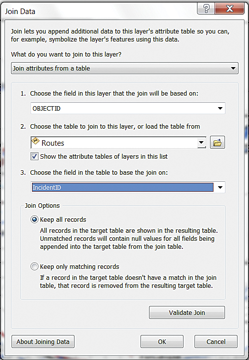
- In the TOC, right-click 2010 Incidents and choose Joins and Relates > Joins. For Item 1, select OBJECTID.
- For Item 2, specify Redlands CF Base Case > Routes. Be sure to specify Base Case.
- For Item 3, select IncidentID. Click Validate and, when validation is complete, click OK to join. Don't index (because you are joining to an active Network Dataset, indexing does not work).
- To build the second join, right-click again on 2010 Incidents and choose Joins and Relates > Joins.
- For Item 1, select FacilityID.
- For Item 2, select Fire Stations.
- For Item 3, select Index. Validate and click OK again. This time, indexing will work, so allow indexing.
- When the second join finishes, open the 2010 Incidents table and verify that Base Case Routes and appropriate station data have been successfully joined to all incidents. If the join was not successful, remove all joins and try again.
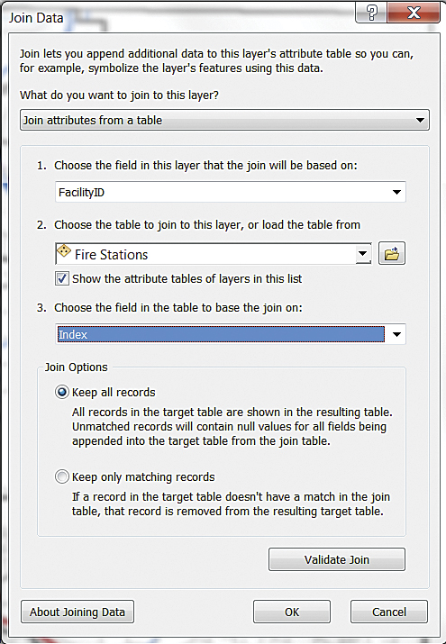
For the second join, set Item 1 to FacilityID, Item 2 to Fire Stations, and Item 3 to Index.
Calculating Travel Times
- To calculate the closest base case stations and travel times for all incidents, open the 2010 Incidents attribute table and locate the Station_Base and Time_Base fields. Right-click Station_Base, select Field Calculator, and click Load. Navigate to \Redlands_Fire, open Station_No.cal, and click OK. Watch as ArcGIS assigns the closest Base Case stations to all incidents.
- Next, right-click Time_Base, select Field Calculator, load Total_Minutes.cal, and click OK to post Base Case travel times.
- Finally, right-click 2010 Incidents in the TOC and select Joins and Relates > Remove Join(s) > Remove All Joins. This is an important step. Do not skip it.
![Select or type [Time_A] – [Time_Base] in the calculation window and click OK.](graphics/stationlocation_9-lg.jpg)
To calculate the time change between Base Case and all incidents modified by response from Proposed A, select or type [Time_A] – [Time_Base] in the calculation window and click OK.
Joining and Calculating the Scenarios
Now that the closest station and travel time have been calculated for Base Case, the same procedure will be used for each scenario. The only difference will be that in the first join, Item 2 will change (e.g., Redlands CF Prop A > Routes, Redlands CF Prop B > Routes, and Redlands CF Prop B > Routes). Although the workflow becomes a bit tedious now, it is critical to proceed carefully. Make the two joins for each layer, successively calculate the Station_A, Time_A, Station_B, Time_B, and Station_AB and Time_AB fields, making sure to remove all joins after calculating the stations and time for each scenario. Carefully check the calculations and save the project. If one or more joins/calculations did not work, clear and rebuild the necessary join and recalculate.
Calculating Travel Improvements

In the First Due Station Group, turn on 2010 Base Case and inspect the incident distribution.
With Base Case and scenario times for all analyses, you can use the Field Calculator to calculate the Change_A, Change_B, and Change_AB fields that are currently filled with zeros in the 2010 Incidents attribute table.
- In the 2010 Incidents table, right-click Change_A and choose Field Calculator. To calculate the time change between the Base Case and all incidents modified by response from Proposed A, select or type the expression
[Time_A] – [Time_Base]
in the calculation window and click OK.
If the Proposed A station, located in northeastern Redlands, can access a 2010 incident before the closest Base Case station, this field represents the time differential as a negative number. If Proposed A is not the closest station, the number will remain zero. If you were modeling closed or relocated stations rather than proposed stations, this number might be positive, representing the additional time required to access an incident, compared to an earlier location. - Calculate the time differential for Scenario B and Base Case in field Change_B, modifying the expression:
[Time_B] – [Time_Base]
Negative values in this column represent improved responses from the Proposed B location in northwest Redlands. - Finally, calculate the combined effect of Proposed A and Proposed B by right-clicking the Change_AB field and modifying the expression to read:
[Time_AB] – [Time_Base] - Sort and review the differential times to see that some incidents improve, while many remain unchanged. Since you have not removed any stations, no incidents display positive values that represent a net travel time increase. Save the map.

Individually open the Travel Time Improvement Group series. This shows effects of Proposed A plus Proposed B.
Mapping
Look at the results on a map. There are many ways that you could map and chart these time-based analyses. A rather basic map would plot closest stations to all incidents for each scenario. Because you have assigned a station number to all incidents, you can readily map this relationship. Station_ field is an integer. Proposed A is designated as 901 and Proposed B is designated as 902. A second map series can show the time change between the Base Case and the three scenarios. You can use a graduated size and color scheme to show how much time is gained or lost as stations open, close, or move. The fields holding differential calculation times contain necessary double precision values.
Inspect the analysis results. Notice the average times for fire responses, EMS calls, and service calls.
- Now you can load the layer files for First Due Station Group and Travel Time Improvement Group. Click the Add Data button and navigate to \Redlands_Fire\GDBFiles\CASP835F to add these groups and quickly create several map series. Position the two groups in the TOC just below Fire Stations.
- In First Due Station Group, turn on 2010 Base Case and inspect the incident distribution. Notice how incidents in differing colors cluster around closest stations.
- Individually turn on 2010 Proposed A, 2010 Proposed B, and 2010 Proposed A, B. Individually open the Travel Time Improvement Group series to show the time decreases for Proposed A, Proposed B, and Proposed A plus Proposed B. Green is good; this is the kind of information that the fire chief and commissioners like to see.

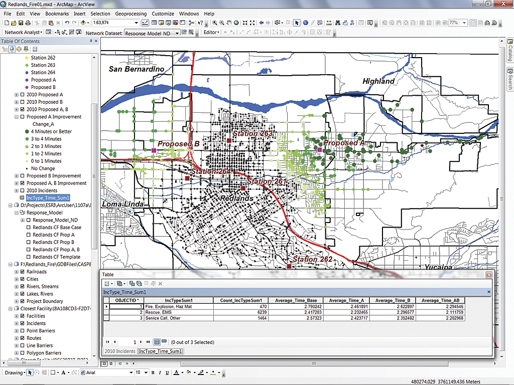
Return to the 2010 Incidents table and locate the IncTypeSum1 field. Right-click this field and select Summarize. Save the summary table in Fire_Data.gdb and calculate average times for Time_Base, Time_A, Time_B, and Time_AB.
Summarizing
Finally, summarize the Base Case and Scenario times for different incident types. Open the 2010 Incidents table, right-click the IncTypeSum1 field, and choose Summarize. Under Item 2, expand Time_Base, Time_A, Time_B, and Time_AB and check the Average box under each. Under Item 3, save the summary table as IncType_Time_Sum1 in Fire_Data.gdb. Add the resultant summary table to the map.
Inspect the results and notice the average times for fire responses, emergency medical service (EMS) calls, and service calls. The proportions and time trends in this table are not unusual. More than 75 percent of all 2010 responses were EMS or rescue calls and average times for these calls are typically the shortest. Nearly 18 percent of all calls are classified as service calls or other calls. Fire and related calls comprise less than 6 percent of all responses. Check out the average times for your scenarios. The average modeled travel time for Proposed A plus B is closing in on two minutes.
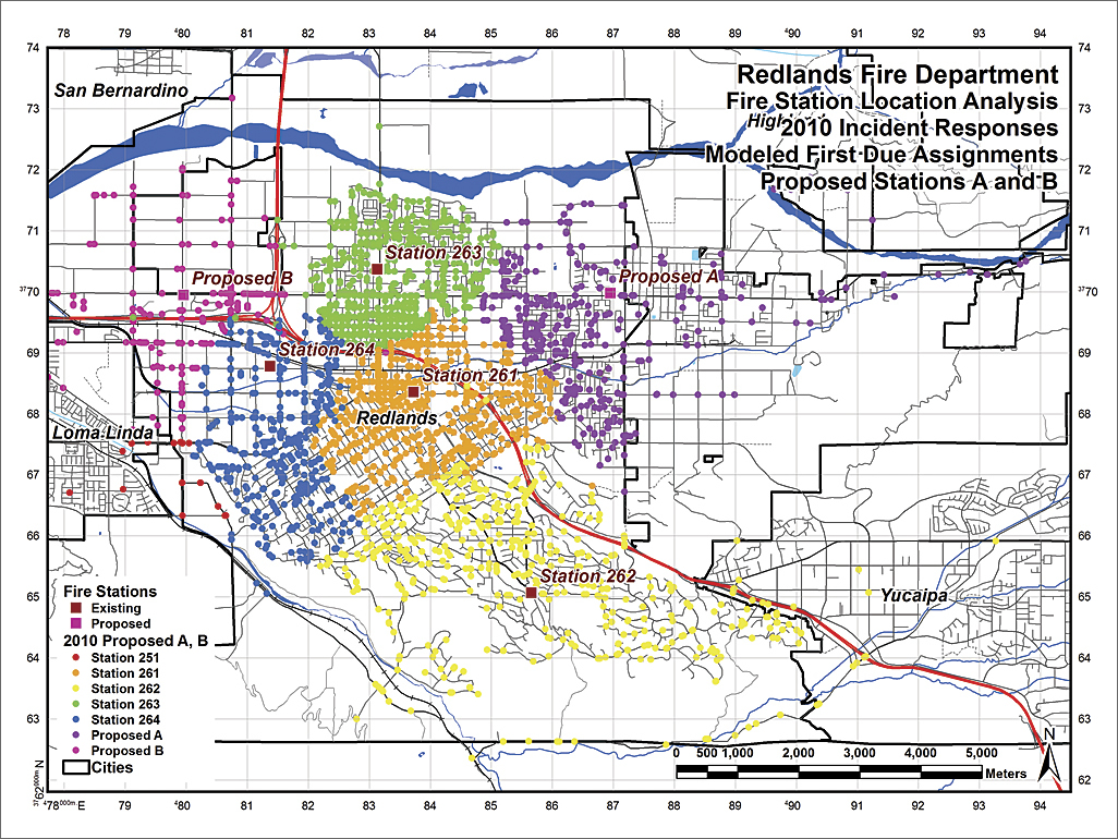
Final map showing modeling of 2010 incident with both Proposed A and Proposed B stations
Future Opportunities
You have only scratched the surface of emergency services modeling. There are many more analyses, maps, charts, and determinations that could be prepared with this data. For a challenge, experiment with actual station relocation or removal. For example, try removing Station 263, located between Proposed A and B, and see how times increase and decrease. Also, experiment with charting in ArcGIS or your favorite spreadsheet program to graphically display the changing data. This is a training dataset, so use your imagination and have fun.
Acknowledgments
Thanks to the fine staff of Redlands Fire Department and City of Redlands GIS for providing this very interesting and complex dataset. Thanks also go to the Confire Communications Center dispatch center for the opportunity to use its excellent time-based streets network in this exercise. The Redlands Fire Department will use many of the same methods and procedures presented here to model and analyze historic, current, and future protection capabilities. Redlands and Esri are very fortunate to have the high level of emergency fire and medical response provided by the Redlands Fire Department.