ArcUser Online
Spring 2011 Edition
Population Drift
Analyzing the location of population centers over time
By Joseph Kerski, Esri Education Manager
This article as a PDF.
What You Will Need
- ArcGIS Desktop (ArcView, ArcEditor, or ArcInfo license level)
- Population Drift: Mean Population Center Analysis lesson downloaded from edcommunity.esri.com/arclessons
- The spatial statistics tools in ArcGIS give you new ways to look at your data.
Examining geographic phenomena using mean centers is a powerful tool in spatial analysis. Imagine your data is on a sheet that is balanced on the tip of a pencil. The mean center is the point at which a given set of features is balanced. The mean center is constructed from the average x- and y-values that are stored in feature centroids.
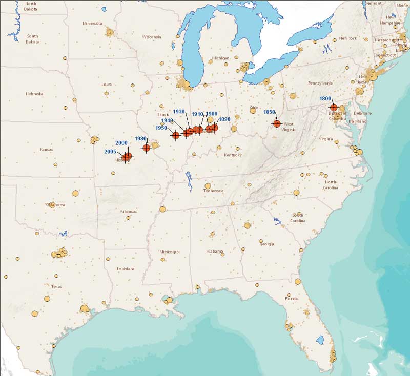
Figure 1: The mean center of population in the United States has shifted over the past two centuries.
The ability to apply weights to the mean center in terms of one or more variables inherent in those phenomena makes the incorporation of mean centers even more useful for instruction and research. The formulas for the mean center and weighted mean centers are shown in Figure 1.
Changes in the mean center of a certain phenomenon can be analyzed over time. Perhaps the most common application for this analysis is the study of the movement of the population center of the United States from 1790 to the present. Maps of this phenomenon appear in many geography textbooks. Computing mean center is easy to do in ArcGIS Desktop because this functionality is part of the spatial statistics tools in ArcToolbox.
About This Exercise
This article provides an introduction to the concept of mean center analysis as it is applied over time and space to a historical dataset. It uses the sample dataset from a tutorial entitled Population Drift: Mean Population Center Analysis, available from ArcLessons. More detailed information and other examples are included in this lesson.
Both article and lesson use the Mean Center tool in the Spatial Statistics Tools toolbox to create mean centers, weighted mean centers, and population mean centers. The results are used to create a map of population center movement in the United States. Intermediate GIS skills are required for this exercise. They may be used in teaching classes from secondary to university graduate level. The 100 questions in the ArcLesson can be completed as an independent study or in a classroom setting and require about three hours to complete. With discussion and deeper analysis, this time frame can be extended to five hours.
These materials teach how to calculate weighted mean centers, select and export spatial and attribute data, and use GIS to make informed decisions. The ArcLesson also encourages additional analysis and provides insights into the causes and effects of population dynamics, including age structure, lifestyle, job growth and decline, rural-to-urban migration, sun belt and retiree migration, and other factors. It also considers the location of lakes, rivers, highways, and federal lands and how they might influence population change.
Computing the Mean Geographic Center for 50 States
Start analyzing the movement of the mean center of population by calculating it for 1790.
If the 50 United States could be balanced on the end of a pencil, in which state would the mean center be? Test your hypothesis by using the directions in the following section to compute the mean center for the 50 states with Shape_Area as the weight field, storing the result in your popcenters_lesson geodatabase (gdb).
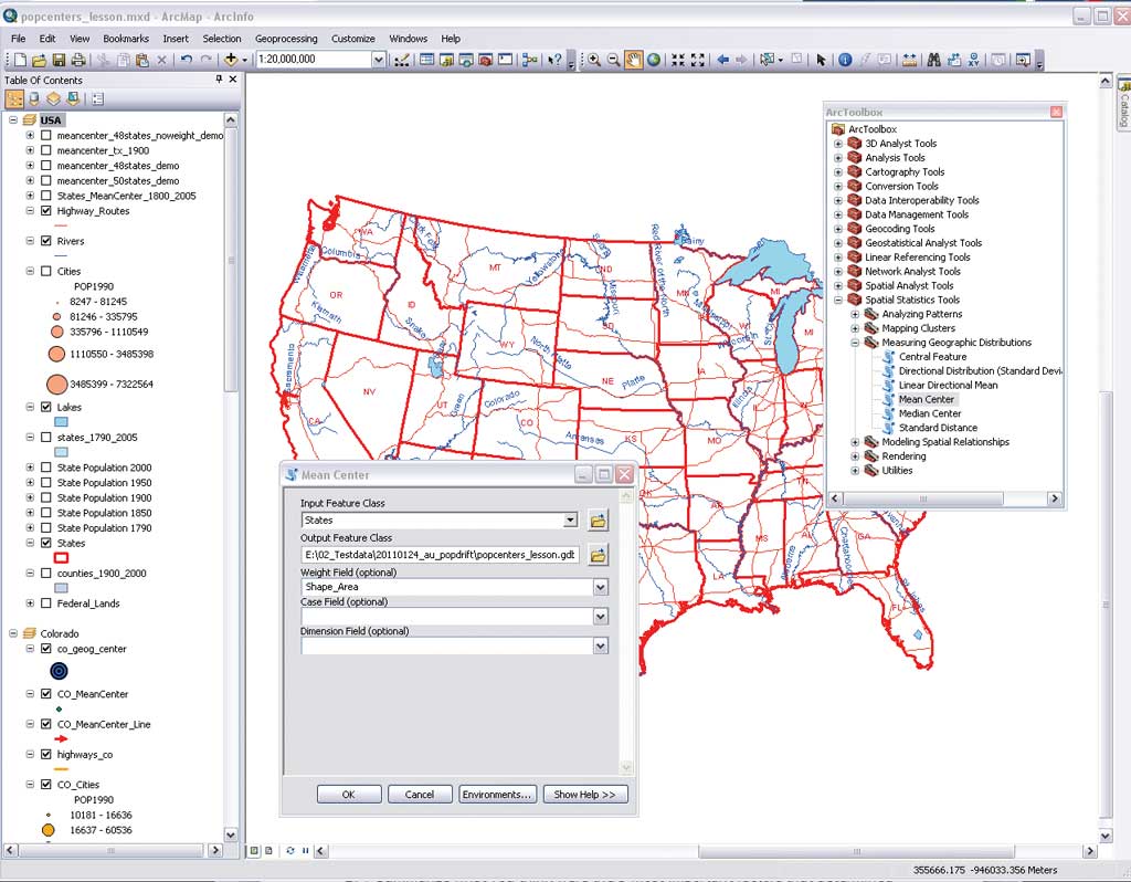
After downloading and unzipping the Population Drift exercise archive, start ArcMap. Open popcenters_lesson.mxd and open ArcToolbox. As you look at this map, consider how the projection used to display a dataset can affect the calculation of the location of the mean center. Is the map projection chosen a suitable map projection to use for calculating mean centers?
In the Spatial Statistics Tools toolbox, choose Measuring Geographic Distributions > Mean Center. Use States as the input layer and Shape_Area as the Weight Field. Store output in popcenters_lesson.gdb as meancenter_50states. During processing, ArcGIS will warn you that the input feature class does not contain projected data, but the tool should execute. Using the Shape_Area field ensures that you are calculating a mean geographic center rather than a mean based on the location of the state centroids. The results are added to the map.
Calculating the Mean Center for 48 States
Next, calculate the mean center for the 48 contiguous states and compare your result to that for the 50 states. Then run the mean center tool for the 48 states but leave the weight field blank, which will simply calculate the mean center of all the features you are analyzing. The mean center without a weight field will determine the mean center of the centroids for those polygons.
- Choose Bookmark > 48 States to zoom to this preset extent. Select the 48 states and rerun the Mean Center tool to calculate the mean geographic center for the lower 48 states. Choose Selection and check States to make sure that only that layer is selectable.
- Click the Selection tool and select the 48 states. (Note that the state "equivalent" Washington, D.C., is also selected, but its area is small and has a negligible effect on overall mean center calculation.)
- Rerun the Mean Center tool using Shape_Area for the weight field. Store the results in the same geodatabase with the name meancenter_48states. In what state is the calculated mean geographic center for the 48 states?
- Run the Mean Center tool for the 48 states, but leave the Weight Field blank. Running the Mean Center tool without anything in the weight field will calculate the mean center of all the centroids for all those polygons. Save the result.
- Compare the unweighted mean center of the 48 states to the weighted mean center and think about how the sizes and locations of the states in the eastern part of the country versus the western part affect the location of the unweighted mean center.
Analyzing the Movement of the US Mean Center of Population, 1790–2005
The mean centers just calculated are based on the total land area for each state. Now look at the population for each state. States have always differed widely in total population. Let's compute the mean population center, which is a center weighted on the population for an area, such as a state.
A mean center weighted on population therefore represents the point location at which a given area could be balanced, based on population. If one state contains more people than another state, the weighted mean population center will be weighted toward, or drift toward, the more populated state than to other states.
- In popcenters_lesson.mxd, turn on the State Population 1790 layer. If the 1790 population of the United States could be balanced on the end of a pencil, in which state do you think this weighted mean population center would be?
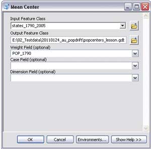
- Calculate the weighted mean population center for 1790 by running the Mean Center tool again, Use the states_1790_2005 layer as the input feature class, use POP_1790 for the Weight Field, and store the result as meancenter_1790 in the same geodatabase.
Changes in Mean Population Centers over Time
- Let's look at the pattern of population change on the map from 1790 to 2000. Turn on and off the map layers showing the state population in 1790, 1850, 1900, 1950, and 2000—one at a time.
- Open the attribute table for the states_1790_2005 layer. Right-click each year field and choose Statistics to obtain additional insights to the changes in population over the centuries. Several fields begin with CHG. These fields contain the percent of change between different census years.
- Run the Mean Center tool six times using the years 1800, 1850, 1900, 1950, 2000, and 2005 using states_1790_2005 as the input layer and the same geodatabase as the output. Name the resultant layers meancenter_
using the appropriate weight fields for the same year (i.e., POP_1800 for 1800). The result will be the population center for each year. - To check your calculations, refer to the USA Population Center Movement graph in Figure 2.
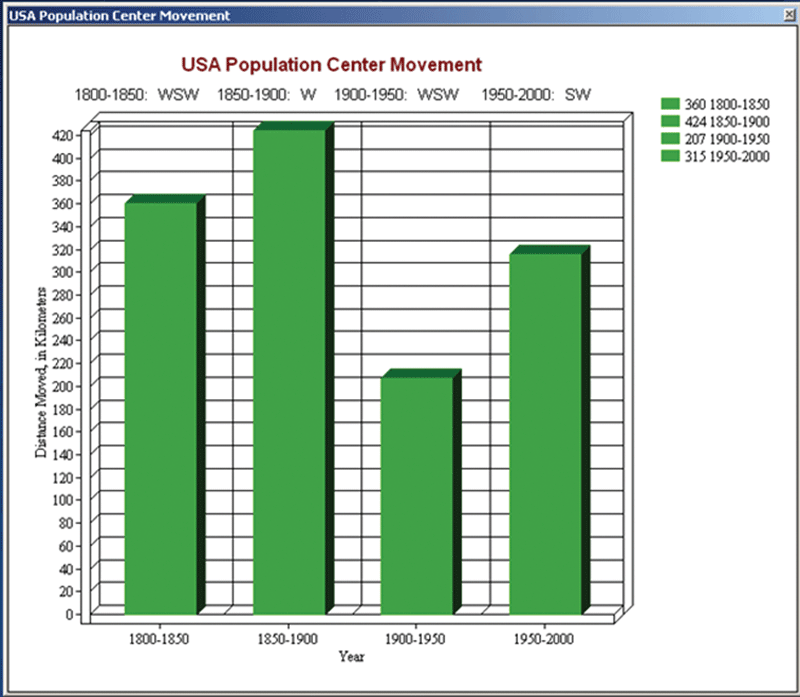
Figure 2: Use USA Population Center Movement to check calculations on mean center movement.
Looking at Population Shifts within States
After looking at population shifts in the United States as a whole, compute population centers for individual states.
County-level data is used to determine the movement of the mean population center within individual states rather than city boundaries because city limits change much more frequently than county lines. While some counties did split off from other counties and others merged or changed boundaries, overall, county boundaries changed much less frequently than city limits from 1900 to 2000. For state-by-state analysis, 1900 is the earliest year examined, because prior to 1900, many county lines were different or nonexistent, and therefore, the geographic framework we need for the analysis wasn't in place.
Using Shape_Area as the weight field ensures that mean geographic center is being calculated rather than a mean based on the location of the state centroids.
The ArcLesson examines mean population center drift for Kansas, Colorado, and Nevada. However, this article looks only at Kansas from 1900 to 2000 and explores which direction the mean population center moved and why.
To explore population shifts over time in Kansas, activate the Kansas data frame. In 1900, Kansas was still being settled by the pioneers who had traveled there by wagon a generation before and now were arriving by railroad, drawn by the promise of cheap land. It was still heavily dependent on the major activity that had attracted most settlers to the state in the first place—agriculture. Initially, eastern Kansas was settled by immigrants from the eastern United States, followed by the settlement of western Kansas.
As the twentieth century wore on, several things happened to slow the population of the central and western agricultural areas in particular. First, the Dust Bowl of the 1930s caused many people to leave the state or abandon agriculture and move to larger towns and cities. Second, the rise of agribusiness and the decline of family farms meant that fewer people were required to live on agricultural lands. Urban areas in Kansas became more diverse. Aerospace companies located in Wichita, and vibrant college towns such as Lawrence and Manhattan continued to attract people to the state, but at a slower rate than for other states.
The map thematically maps population for cities and counties. The mean center of population in Kansas is shown by the red line in east-central Kansas in more detail, moving west, then reversing direction to head east.
Analyzing Mean Population Centers for Other States
You can analyze the movement of mean population centers over time for other states without clipping the counties and other layers and placing them in separate data frames. These steps describe how to analyze another state, Texas, using Select By Attributes.
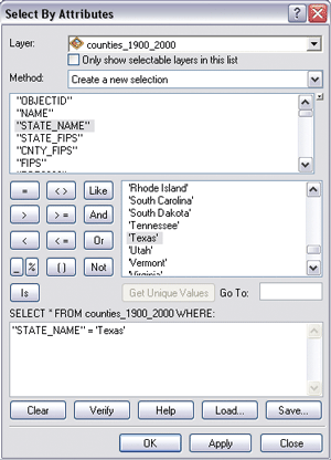
Use Select By Attributes to analyze the movement of mean population centers for individual states without clipping data.
Activate the USA data frame. Choose Selection > Select By Attribute. In the dialog box, choose counties_1900_2000 for Layer and Create a new selection for Method and create the expression "STATE _NAME" = 'Texas' in the text box.
Run the Mean Center tool for 1900 for Texas using counties_1900_2000 as your input layer. Write the result to the same geodatabase and name the output feature class meancenter_tx_1900. View the mean center that has just been calculated by adding the meancenter_tx_1900 layer to the map. Run the mean center tool once more for each census year: 1910, 1920, 1930, 1940, 1950, 1960, 1970, 1980, 1990, and 2000.
After running the Mean Center tool for each census year, the related ArcLesson encourages the student to describe the spatial pattern of cities, highways, rivers, and federal lands and population in 2000 by county in this state as well as conduct some research about the settlement, economy, and population of Texas from 1900 to 2000 to examine why the mean center of population moved from 1900 to 2000.
Exploring More
The ArcLesson Population Drift: Mean Population Center Analysis provides more questions for exploring this data using the Mean Center tool in the Spatial Statistics Tools toolbox. Questions posed in the lesson invite a detailed analysis of the change experienced by each state. The lesson contains 100 questions that can spark discussion and new lines of questioning.
The mean center can be calculated from point, line, or polygon features and used for many types of analyses. The mean center of a set of soil samples, the mean center of asthma patients in a city, and the mean center of gas wells in a basin are three of a myriad of types of data that could be analyzed using these easy-to-use but powerful tools.