ArcUser Online

Relief Mapping
   Real-World Challenges

by Jim Mossman, Data Deja View

Editor's note: An article, "New Color System Enhances Relief Mapping," in the October–December 2000 issue of ArcUser magazine introduced the DDV ShadeMax Color Palettes, a set of color palettes and legends that simulate continuous change in color with elevation. These palettes were developed by Jim Mossman for use with ArcView GIS and the ArcView 3D Analyst and ArcView Spatial Analyst extensions. In this article, Mossman describes the steps used to create a beautifully shaded relief basemap of Wyoming. He not only explains how to customize ShadeMax color palettes for this particular map but also describes the process he used to acquire and manage the data for this map and design its layout.

Software, Data Sets, and Hardware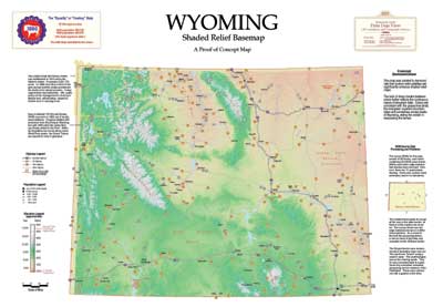

This map was produced with ArcView GIS 3.2 and the ArcView Spatial Analyst and ArcView 3D Analyst extensions. Data import, projection, and overlay tasks were performed using ArcToolbox, one of the ArcInfo 8 desktop applications. However, those tasks could have been carried out using ArcView GIS. Two extensions, XTools and Spatial Tools, a script, Grid.ClipToPoly, and a set of color palettes, the DDV ShadeMax Color Palettes, all available at no charge from the Esri ArcScripts (arcscripts.esri.com), were also used to process data and design this map. The ShadeMax color set consists of 12 main palettes of closely grouped color schemes for use in graduated color legends, 12 thematic prebuilt legends that can be used as is or as templates, and an ArcView GIS project containing a layout and several custom legends and instructions. These templates help users create ArcView Spatial Analyst and/or ArcView 3D Analyst legends for specific needs.

Sources of data for this map included the University of Wyoming's Spatial Data and Visualization Center (SDVC) and the Digital Atlas of the Greater Yellowstone Area. SDVC provides more than 500 spatial data sets that can be downloaded from the Web site. The Digital Atlas of the Greater Yellowstone Area contains 275 layers including data on topography, geology, water resources, wildlife species, roads and trails, and demographic and economic information that can be downloaded or obtained in CD̫ROM format.

The elevation grid used was built using digital elevation model (DEM) data created by the United States Geological Survey (USGS). Fifty-six blocks of 32 quadrangle maps each-or a total of 1,792 quads-were used. However, 30-meter DEM data was not available for 11 quads. The blocks containing these quads were projected in Universal Transverse Mercator, Zones 12 and 13. The westernmost blocks did not go all the way to the State border. Unzipped e00 block files were imported into two instances of ArcToolbox, and the runs were overlapped. Block projection changes were specified in two ARC Macro Language (AML) scripts and were run in concurrent Arc sessions. Both Dell processors averaged 90-100 percent utilization, illustrating the benefit of using computers with dual processors when working with multiple, large data sets in ArcInfo. Mosaicking of the blocks into a State-wide grid was done in several steps in ArcView GIS using the Spatial Tools extension.

The large data sets used for this map seriously challenged the author's hardware. A Dell Precision 410 with dual 400 MHz processors, 512 MB of RAM, and a 32 MB Diamond Fire GL1 AGP video card running on Windows NT 4.0 with Service Package 6a was used for processing and mapping data. Printing was done on an Epson Stylus 3000 at 720 dpi using both Epson drivers and ArcPress for ArcInfo.

Shading the Basemap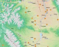

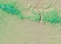
This map showcases the benefits of tailoring color application to meet special mapping needs. Customization included adding new colors to the palette and not applying some colors uniformly with elevation. SM05 Wyoming Territory, one of the 12 ShadeMax color palettes composed of five subgroupings, was used for this demonstration. Using the ArcView Spatial Analyst extension, USGS DEM files were imported as grid files and a hillshade created by choosing Surface > Compute Hillshade from the View menu. The following steps detail how the SM05 palette was customized to the Wyoming data sets.

1. Using the Legend Editor, the grid was initially classified with 43 equal intervals and the original SM05 base colors were applied sequentially. White was used for the last interval. The hillshade was then added as a brightness theme by clicking on the Advanced button in the Legend Editor. In the Advanced Options dialog, the Wyoming hillside was selected from the drop-down box as the brightness theme, and the minimum cell brightness was set to 50 and the maximum cell brightness was set to 100. Clicking OK applied these settings.
2. To make the mountains stand out more, the number of classes was increased, elevation ranges were adjusted, and the palette colors reapplied using the Legend Editor. White was applied to the 14 highest elevation ranges by clicking on the first range, holding down the Shift key, clicking the last block in the range, and selecting white from the Color palette. Such biasing of colors may be necessary to emphasize important features that otherwise do not show to the desired degree. Close inspection of the lowlands revealed many features that were not showing up well. To correct this, slightly more contrasting colors were added to the palette for use in the lower elevation ranges.
3. After inspection, the grid classes were again increased and individual elevation range values readjusted. SM05 base colors were applied starting at 1,450 meters through 3,500 meters, and white was used for the higher elevations.

4. A reddish color from another palette was applied to the lowest elevation of the expanded legend by clicking in the symbol field for the lowest range, choosing the new color from the Color palette dialog and adjusting its hue, saturation, and value (HSV) settings manually.
5. Next, the elevation ranges between the new lowest elevation color and the 1,450 through 3,500 meter elevation range were ramped. The ranges between 1,450 meters and 3,500 meters were selected by clicking on the 1,450 meter range, holding down the Shift key and clicking on the 3,500 meter range, then holding down the Control key and clicking on the lowest range.
6. Clicking on the Color Ramp button fills in the missing colors between the selected block and lowest range without affecting the SM05 colors previously applied. Reapply the Hillshade brightness theme as described in Step 1.
7. The legend was saved using the leg2pal.ave script. This script takes the colors from the active theme's legend and copies them to the current Color palette. After the script has executed, the palette still must be saved by clicking on the Save button in the Legend Editor. Because these new colors worked well, the author updated ShadeMax to include them and reposted the improved version on the ArcScripts site.

Customizing the Legend in a Layout

The DDV ShadeMax Color Palettes download contains an ArcView GIS project called Legend_Graphic.apr. This project contains a single layout document with text and graphics depicting several legends for use with ArcView Spatial Analyst. Creating a template that incorporates one of these legends can save time in making an attractive legend.

1. A template containing the Open Legend_Graphic.apr legend was used to create a new layout.
2. The legend in the new layout was selected using the selection tool. The graphic elements making up the legend were ungrouped by choosing Graphics > Ungroup from the Layout menu. The scale in the layout legend was adjusted to match the legend in the view using the line and text tools.
3. The colors in the legend were modified by choosing Graphics > Properties to bring up the Color palette. The legend was customized to match the elevation theme's colors. The palette saved earlier using the leg2pal.ave was used to recolor the left side of the legend.

4. Grayed colors from the original SM05 set were used to recolor the right side between 1,450 and 3,500 meters. Elevations higher than 3,500 meters used the same gray applied to the 3,500 meter range. The right column's lower elevation colors were created with the Custom color button using left column colors less than 50 value units.
5. Spot checks of the map's elevation grid were made to ensure legend colors and elevations were correctly associated. While this process involved some tedious, close-up detail work, none of the steps were difficult.

About Legend Accuracy

The underlying goal was to use elevation colors so close together that shaded relief appears seamless. Viewers would only be able to approximate map elevations, so minor scaling inaccuracies in constructing the legend would be acceptable. If more exact elevation identification is necessary, contour lines and/or spot elevation labels can be used.

Grid to TIN and Back

ArcView 3D Analyst was used to convert the grid to a TIN and fill in the vacant quads, using 5 for the z value. After almost three days of churning, while facing a deadline, the run was stopped and the TIN added to the view. The TIN was then converted back to a grid. In the resulting theme, the triangles generated across gaps became visible only when zooming in on the theme in those areas. Allowing the TINing to continue might have made these triangles smaller.

ArcView 3D Analyst was used to convert grid data to a TIN to fill in the missing quad data.

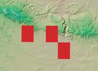
Large triangles did show in the dish created by the Lambert projection along the top of the State. The Grid.ClipToPoly script was used to convert that area to No Data values. Though this process gave outstanding results for the State-wide map, the final grid is obviously not suitable for analysis or smaller area mapping in the vicinity of the missing quads.

On Map Design

After all the processing was completed, the desired map components were roughly defined and sketched so that good combinations of size and placement could be identified. While it was tempting to make the area occupied by the State bigger, blank areas are important to the design. Placing two map components in small rectangular areas at top left and right of the map balanced the large rectangular mass of Wyoming that was centered toward the bottom of the map to accommodate the title block.

Using the ShadeMax palettes and tweaking the color by adding additional shades and refining the assignment of elevation values to colors enhanced this relief map. These simple tools and concepts can give new usefulness to relief maps. The author hopes this example inspires others to innovate. Using a different approach and a custom touch in meeting mapping challenges can be especially rewarding. For questions about these maps contact the author at jmossman@wcvt.com.

Return to Table of Contents for April–June 2001 issue