ArcUser Online

Answering Real-World Questions

Using 3D volumetric analysis techniques in ArcGIS 10

By Nathan Shephard, ArcGIS 3D Analyst Visualization Product Engineer Lead

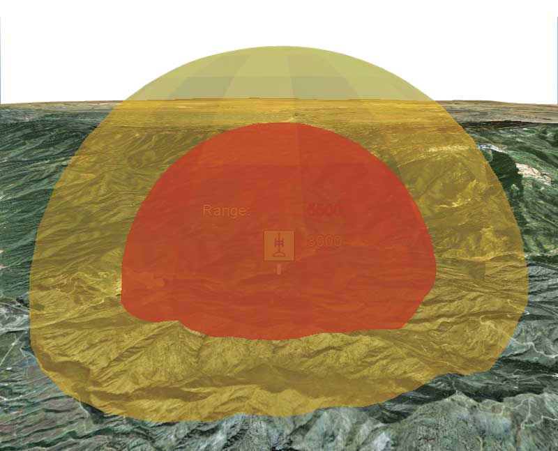
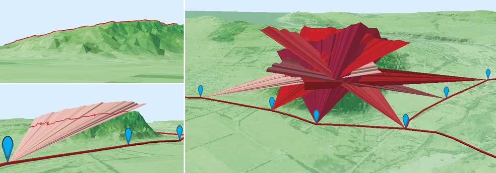
See original animation that triggered this article.

An antiaircraft gun point feature has been symbolized as two threat dome layers—one with a 5,500-meter radius and the other with an 8,000-meter radius.

The threat dome has been trimmed by the visibility volume for the antiaircraft gun.

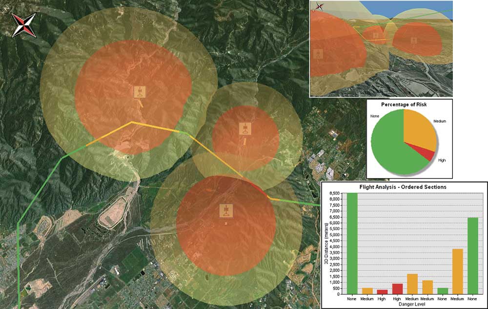
The 3D flight route has been intersected and classified based on the threat volume that contains it. Information can be summarized into graphs. This example has one graph summarizing the overall risk (A) and a second one that displays the flight path as ordered stretches of risk (B).

This article as a PDF.

Some geographic questions can only be answered in 3D. Which offices in a building are close to these stored dangerous materials? How much water will fit inside this valley? Will my backyard suntanning days be over once that new building is finished?

Intersect 3D, Inside 3D, and Skyline Barrier are some of the analytic tools that were added to the ArcGIS 3D Analyst extension at version 10 specifically for working with GIS data in true volumetric space. This article illustrates how these new tools can be used to answer 3D GIS questions by stepping you through the process of performing two analyses that use techniques with broad applications. The key point in the specific use cases cited in these examples is that 3D GIS tools are generic and can be applied to solve a wide variety of problems. Just as the Buffer tool can have many applications, the Intersect 3D, Skyline, and Skyline Barrier tools can be used to provide answers to many different kinds of questions.

Example 1: Avoiding Dangerous Airspace

The first question we'll investigate using these new tools in 3D Analyst is, How risky is this flight through dangerous airspace? While this is obviously a military example, it's not too difficult to imagine that techniques for analyzing the intersection of a flight path with dangerous airspace could be applied to the analysis of other problems such as locating an underground pipe away from planned subsurface drilling or assessing the potential effects of vibrations caused by a proposed subway on the residents of nearby homes.

Pilots don't want to be targets and try to avoid routes where they are likely to be fired upon. Identifying the sections of a planned route where this kind of thing could happen can make or break a mission. This is an inherently 3D problem, because the ranges calculated for weapons are often based on direct 3D distances.

Certain base data is required to analyze this problem: an elevation surface, the proposed flight path, locations of threats, and information about the effective range of each threat. To translate these requirements into GIS terms, you will need an elevation surface such as a raster digital elevation model (DEM), a triangulated irregular network (TIN), or a terrain dataset; a 3D line feature class that describes the proposed route(s); and a 2D (or 3D) point feature class that contains attributes for threats. This example uses a 5-meter raster DEM.

In the first step, the 2D point features are converted to quantifiable threat domes. This example has three antiaircraft (AA) gun positions. Each AA gun has different effective ranges depending on the presence or absence of radar assistance. The outer zone (where radar assistance is required) is less dangerous than the inner zone because the plane's countermeasures are more effective.

This information can be converted into threat domes (which are more easily understood) using feature attributes to drive the construction of threat dome features using the following workflow.

In the ArcScene application in 3D Analyst, add the point feature class twice to create two layers in the table of contents.
Set the symbology for each layer to Simple Marker Symbol > Sphere.
Set the Advanced > Size value for one layer to InnerThreatDistance and the other to OuterThreatDistance.
Use the Layer 3D To Feature Class geoprocessing tool to convert these symbolized layers into volumes and store them as multipatch features in two new feature classes.

Layer transparency and layer rendering priority provide the framework for seeing these nested/overlapping threat domes in a three-dimensional view. Although these threat domes are useful, they do not take into account one of the most useful factors when trying to protect planes from antiaircraft fire—the terrain.

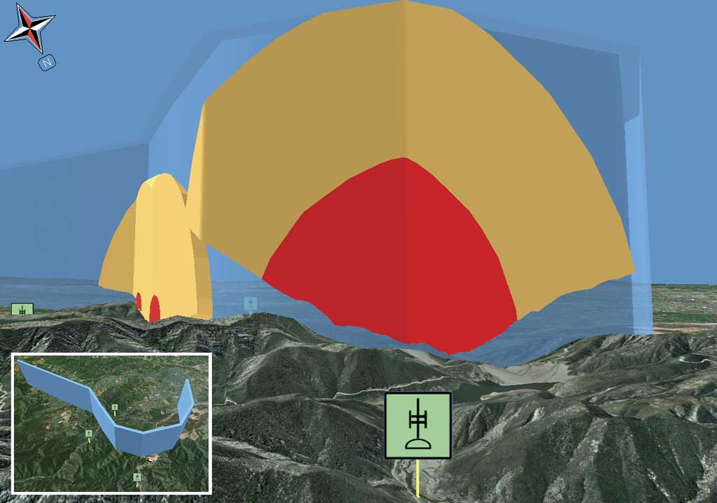
The orange and red volumes illustrate the dangerous airspace within the blue flight corridor.

How tall can the buildings located in the orange area be and still remain unseen from the blue viewpoints?

Use the Skyline and Skyline Barrier tools to calculate a barrier or fan that separates the ground from the sky from each viewpoint.

The Skyline and Skyline Barrier tools can help incorporate terrain into this analysis. The Skyline tool generates the visible horizon for each threat position. The Skyline Barrier tool can effectively project this horizon up into the sky, displaying the results as a volume representation of the visible airspace above each threat point. Intersecting these volumes with the pure distance-based threat spheres generates danger zones that incorporate both visibility and lethal ranges.

To identify which sections of the proposed route intersect the 3D danger zones, use the Intersect Line With Multipatch tool. It splits the route into sections of low, medium, and high risk. The 3D distances of each segment can be easily calculated using the Calculate Geometry option for a field or the Add Z Information tool. This exposes information that will be summarized into graphs. For example, one graph could summarize the overall risk, while another could display the flight path as ordered stretches of risk. Repeating this analysis for multiple proposed routes and comparing the resulting graphs can help select the best route.

Advanced users can expand this analysis by converting the infinitely thin flight paths into volumetric flight corridors. One simple way to do this is to buffer the flight path into a polygon and extrude that polygon between a minimum and maximum altitude range. Using the volume-based Intersect 3D geoprocessing tool (rather than the line-based Intersection tool), all the threat volumes within the corridor can be derived. This provides additional options for accessing flight safety. For example, the north side of a flight corridor could be safer than the south. It also provides a more complete summary of the total dangers associated with a flight corridor.

Note: The 3D volumetric analysis tools can create incredibly complex geometries that can contain hundreds of thousands of triangles, which may exceed the number of operations that can be run. However, this restraint is expected to ease over time as the underlying Computational Geometry Algorithms Library (CGAL) expands.

Flash Player Required

Watch a video illustrating this analysis in 3D Analyst narrated by the author.

Example 2: Hiding Tall Buildings

The second question we'll examine, How tall can these buildings be without being visible from nearby major roads? is a real urban development use case that has been mandated by law in many countries. However, the same workflow could also be applied to other scenarios: placing mining rigs so they can't be seen, finding locations that hide military vehicles from view, or identifying sections of a forest that can be harvested while minimally impacting the appearance of the surrounding countryside.

This scenario is similar to the children's game of hide-and-seek—find a place where it's hard for others to see you. This seemingly simple problem can be challenging to solve using software. However, by thinking creatively, 3D analysis tools can be used to figure out where to hide 3D GIS features. In this example, those features are proposed buildings that shouldn't be visible to drivers on nearby major roads.

Again, the first and most crucial step is acquiring the appropriate data. For this example, that data is an elevation surface, 2D data for the area of interest, and data for the view positions to be protected. In terms of GIS data, that equates an elevation surface (a raster DEM, TIN, or terrain dataset), a 2D polygon feature class containing the area of interest, and a 2D (or 3D) point feature class that describes the view positions. For this example, the elevation data will come from a TIN.

The area of interest is behind a ridge, so the first task is creating a barrier (or fan) that defines the separation between the sky and the ground from each view position. In this example, only the elevation surface is being used to generate the skyline features. If existing structures were in this vicinity, they could also be included in the calculations. The workflow for this example is

Run the Skyline tool using the view-points and elevation surface to create skyline features.
For improved performance, set feature attributes for each viewpoint to limit the sweep of the calculation.
Run the Skyline Barrier tool using the skyline features and viewpoints to create skyline fans.

After calculating the visibility planes, the next step is calculating the 3D space between these planes and the ground in the area of interest. Although there are several ways to run this analysis, one simple method that scales well (because it avoids potentially complex and enormous geometries) is to model the area of interest as vertical lines and slice those lines using the skyline barrier fans as described by the following workflow:

Run Create Random Points to fill the polygon with many point features.
Use layer properties to extrude the points just created into vertical sticks.
Run the Layer 3D To Feature Class tool to convert the vertical sticks into vertical line features.
Run the Intersect 3D Line With Multipatch tool to cut the vertical lines with the skyline fans.

Use the skyline fans to slice vertical sticks within the area of interest.

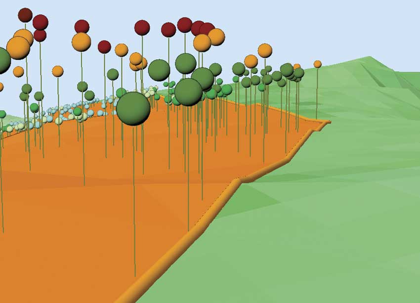
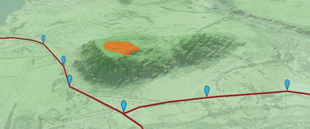
The virtual lines indicate elevations that cannot be seen from the road. The top vertex of each is displayed as a point feature.

The green zones can contain 20-meter-tall buildings that cannot be seen from the road.

Once all the virtual lines have been cut by the fans, the remaining sections represent elevations that cannot be seen from the view positions.

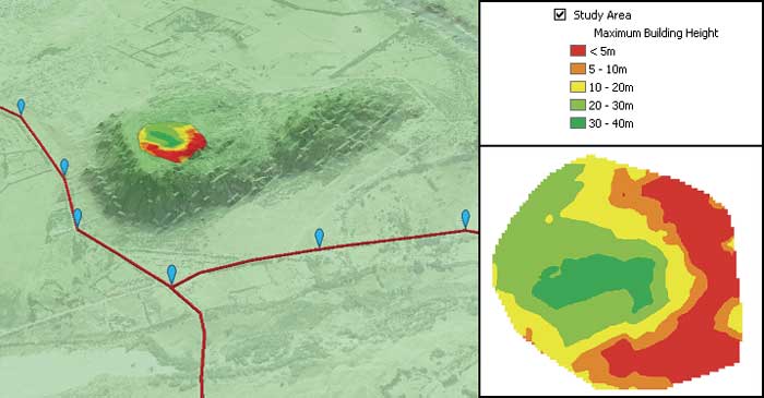
These 3D vertical lines can be converted into maximum height construction zones. The top points can be used to create a new TIN surface using the Create TIN and Edit TIN tools. This surface defines the top of the volume that is hidden from view. Comparing this surface to the base elevation surface using the Surface Difference tool will result in a raster in which each cell value represents the hidden building height for that area.

Displaying this raster output using a simple class-breaks renderer completes the analysis of this problem. This layer can be viewed in 3D or copied into ArcMap and shared as a 2D map. The layer makes it simple to identify where structures of a certain size can be built that while remaining concealed from view on the roads.

Conclusion

The two questions answered in this article were complex. 3D GIS was integral to arriving at the correct solutions. Both were tackled using standard GIS techniques such as attribute-driven symbology, feature intersection, and surface generation. This shows just how far 3D GIS has come with the release of ArcGIS 10. Although you might not be a fighter pilot or the architect of high-rise buildings, you can see from the examples in this article how these 3D techniques can be adapted to solve questions you face. The visibility analysis in the second example is covered in detail as part of the instructor-led Working with 3D GIS Using ArcGIS training course. See training.esri.com for more information on this course.

About the Author

Nathan Shephard has a bachelor's degree in computer science (GIS) from Curtin University in Western Australia. He worked for three years with ESRI Australia before coming to the Esri Redlands campus in 1999.

News