ArcUser Online
Understanding Geodesic Buffering
Correctly use the Buffer tool in ArcGIS
By Drew Flater, Esri Geoprocessing Development Team
This article as a PDF.

Figure 1: The original map showing 10,000 and 15,000 km buffers around North Korea
Several years ago, a major newsmagazine published a map (similar to the one in Figure 1) that showed 10,000- and 15,000-kilometer (km) ranges for missiles launched from North Korea. If you lived in Europe, the Americas, or most of Africa and were not familiar with earth's dimensions, this map might have been comforting because it appears that those areas are outside the reach of even the longest-range missiles launched from North Korea. However, if you are familiar with earth's dimensions, you might have noticed something wasn't quite right with this map.
Earth's circumference is approximately 40,000 km. A 15,000 km buffer would result in a circle with a diameter of 30,000 km. Yet the buffer shown on this map covers far less than three-quarters of earth's 40,000 km circumference. Something was definitely off.
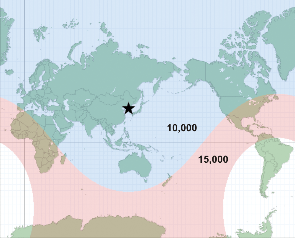
Figure 2: The corrected map showing 10,000 and 15,000 km buffers around North Korea
Figure 2 shows a corrected map that was published by the magazine two weeks later. In the corrected map, all of Europe, Asia, and most of North America are within the 10,000 km range, and only South America is outside the 15,000 km range. What went wrong with those original buffers? Could the analyst have entered the wrong buffer distances? The answer is not quite that simple.
Understanding Buffering
The Buffer tool, a geoprocessing tool in the Analysis toolbox in ArcToolbox, generates buffer polygons, or offsets, around input features at a specified distance. Buffers show the area that is within some distance of the input features. The tool is popular because the concept of buffering is easy to understand and buffering plays an important role in many geoprocessing workflows involving proximity or distance analysis (i.e., How far away are these things? or What features are within a distance of other features?). Because the Buffer tool is important in performing proximity tasks, a key goal for developers working on this tool has been to ensure that buffers accurately depict distances around features.
The Buffer tool is used when analyzing data from many sources—from national forest inventories to local street centerlines. However, a better understanding of how this tool works is necessary to ensure that analysis results are reliable.
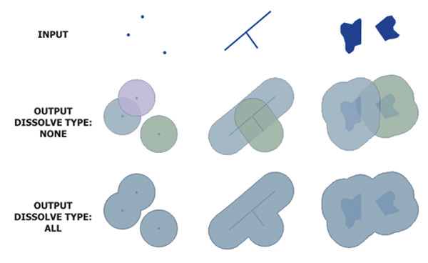
Figure 3: How the Buffer tool creates line and point buffers
Euclidean and Geodesic Buffering
The ability to generate geodesic buffers is an important feature of the Buffer tool that can help prevent the kind of mistake made by the analyst mapping those missile ranges. Geodesic buffers account for the earth's actual shape in the calculation of the buffers. The earth is an ellipsoid (or, more properly, a geoid), and when the Buffer tool generates geodesic buffers, distances are measured between two points on a globe.
Euclidean buffers—another kind of buffer—measure distance on a two-dimensional Cartesian plane. With Euclidean buffers, straight-line distances are calculated between two points on a plane. Euclidean buffers appear as perfect circles when drawn on a projected flat map, while geodesic buffers appear as perfect circles only on a globe. On two-dimensional maps, geodesic buffers often appear as irregular ellipses.
Euclidean buffers are more common. They work well when analyzing distances around features that are concentrated in a relatively small area in a projected coordinate system (e.g., when all features are contained in one universal transverse Mercator [UTM] zone). Geodesic buffers are less common but provide more accurate buffer offsets for features that are more dispersed (i.e., cover multiple UTM zones, large regions, or even the whole globe).
In some situations, performing a Euclidean buffer will produce results that are not technically correct. In the missile range mapping example, the first map used Euclidean buffers, while the second map used geodesic buffers. The major danger when performing a Euclidean buffer on features stored in a projected coordinate system stems from the distortion of distances, areas, and the shapes of features caused by projected coordinate systems.
For example, when using UTM (a projected coordinate system), features become more distorted the farther they are from the origin of the projection (i.e., the center of the UTM zone). When using a dataset that is not contained in a single UTM zone or when the buffer distance used is large enough to create offsets outside that zone, Euclidean buffers will yield incorrect results.
Similarly, if a world projected coordinate system is used, distortion is often minimal in one area but significant in another. For instance, distortion in the Mercator World projection is minimal near the equator but significant near the poles. For a dataset that has features in both low- and high-distortion areas, Euclidean buffers will be more accurate in the low-distortion areas and less accurate in the high-distortion areas. Geodesic buffers will be accurate in all areas.
Performing Geodesic Buffering
At ArcGIS 9.3, the Buffer tool included the functionality to produce geodesic buffers. To perform geodesic buffering with the Buffer tool, these criteria must be met:
- The input feature class must be a point or multipoint dataset.
- The input feature class must have a geographic coordinate system.
- The buffer distance must be specified as a linear unit such as kilometers, miles, or feet.
To perform geodesic buffering on an input feature class that is a polygon or polyline dataset, first use the Feature To Point tool (located in the Data Management toolbox in ArcToolbox). If the input feature class has a projected coordinate system, use the Project tool (also found in the Data Management toolbox) to make a copy of the feature class in a geographic coordinate system. Enhancements to the Buffer tool being explored for future releases of ArcGIS will allow geodesic buffers to be generated from line and polygon inputs.
Looking at Some Examples
In each of these examples, Euclidean and geodesic buffers are compared with various point datasets in different coordinate systems. Two sets of each point feature class were used to accomplish this effect for each example: a point feature class in a projected coordinate system that was used to generate Euclidean buffers and a copy of that point feature class in a geographic coordinate system that was used to generate geodesic buffers. The buffer distance used for both the Euclidean and geodesic buffers was held constant. In each example, Euclidean buffers are shown as thicker red rings, and geodesic buffers are shown as blue rings.
UTM Projection (UTM Zone 30N; WGS 1984 Datum)
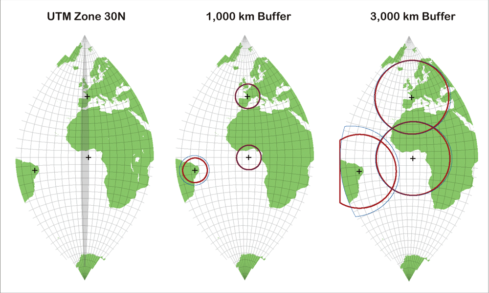
Figure 4: (a) UTM Zone 30N projected coordinate system with a 10 x 10 degree grid, (b) 1,000 km buffers, and (c) 3,000 km buffers. The Euclidean buffers are shown in red, and geodesic buffers are shown in blue.
In Figure 4, 1,000 and 3,000 km buffers are shown on a map in a projected coordinate system, UTM Zone 30N with a 10 x 10 degree grid for reference. Zone 30 is shaded in the first map. UTM zones are roughly 6-degree-wide bands that run north and south between the poles. UTM Zone 30 is the zone immediately adjacent to the prime meridian.
In the 1,000 km buffer graphic, the two points within Zone 30 have Euclidean and geodesic buffers that are coincident. This shows that for points within the zone, the UTM projection does a good job minimizing distance distortion, regardless of latitude. The third point to the west of these two points (on the horn of Brazil) has geodesic and Euclidean buffers that are significantly different.
Outside Zone 30, distance distortions cause the Euclidean buffer to be considerably undersized compared to the geodesic buffer, although that buffer is exactly the same size as the two other Euclidean buffers. This occurs because the Euclidean buffer assumes that map units are the same everywhere in the projection (i.e., 1 km on the horn of Brazil is the same as 1 km in the Atlantic Ocean south of Africa). This is not true, because outside UTM Zone 30, the distance becomes more and more distorted with this projection.
Different-sized geodesic buffers illustrate how the map projection is distorted. Each buffer would be identical in size on a globe. Because all these geodesic buffers have the same area but the geodesic buffer in Brazil looks larger than the others, it can be assumed that the projection is causing features to be stretched out or enlarged in this area.
In the 3,000 km buffer graphic, the Euclidean and geodesic buffers for points inside Zone 30 are beginning to diverge. Although the features are within Zone 30, the buffers extend far outside the zone and cause the Euclidean buffers to be slightly distorted.
Because the dataset includes features outside the target zone and a buffer distance is used that causes the offsets to extend well outside the target zone, geodesic buffers should be used because they more accurately portray the buffered area.
World Projection (World Mercator; WGS 1984 Datum)
When working with a dataset in one of the common projected coordinate systems for the whole world, such as Mercator, projection distortion may be minimal near the equator but significant near the poles. Figure 5 shows 1,000 and 3,000 km buffers on a map with the projected coordinate system Mercator (World).
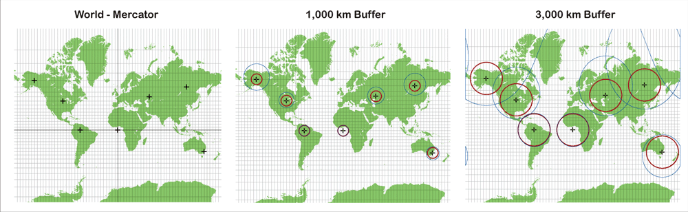
Figure 5: (a) Mercator (World) projected coordinate system, (b) 1,000 km buffers, and (c) 3,000 km buffers. The Euclidean buffers are shown in red, and geodesic buffers are shown in blue.
In the 1,000 km buffer graphic, the points near the equator have geodesic and Euclidean buffers that are coincident. For points near the equator, the Mercator projection does a good job minimizing distance distortion.
Points far from the equator show the most distance distortion. The Euclidean buffers for those points are considerably smaller than the geodesic buffers. This occurs with the Mercator projection because, at the poles, areas are stretched. Land masses close to the poles, such as Greenland and Antarctica, appear to have enormous areas compared with land masses that are actually similar in size but located close to the equator. All 1,000 km Euclidean buffers are the same size because the Euclidean buffer assumes that map units are the same everywhere in the projection (1 km in Brazil is the same as 1 km in central Russia). This is not true, because as locations move away from the equator, the distances become more and more distorted with this projection.
The variation in size of geodesic buffers shows how the map projection is distorted, because each buffer would appear identical in size on a globe. The same results, though exaggerated, are shown in the 3,000 km buffer graphic. With any type of analysis of distance on a global scale, geodesic buffers should be used because (again) they more accurately portray the buffered area.
Conclusion
When performing a buffer operation with a dataset that has features covering a large region or when using a very large buffer distance, it is important to remember that projection distortion can have a serious effect on the results. In both cases, Euclidean buffering performed on projected feature classes can produce misleading and technically incorrect buffers. However, geodesic buffering will always produce results that are geographically accurate because geodesic buffers are not affected by the distortions introduced by projected coordinate systems.
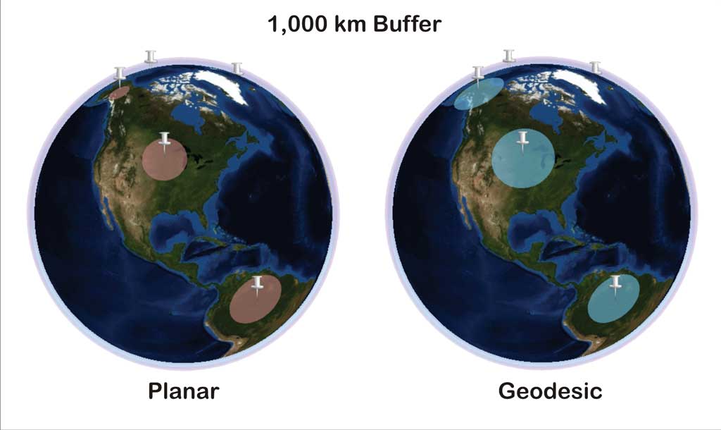
Figure 6: Euclidean (shown in red) and geodesic buffers (shown in blue) in ArcGlobe
Displaying buffers in ArcGlobe or ArcGIS Explorer can help visualize the problems that occur when buffering projected data because these applications can display geographic data on a three-dimensional globe. Figure 6 shows the same 1,000 km Euclidean and geodesic buffers shown in Figure 4, displayed in ArcGIS Explorer. When displayed on a globe, these Euclidean buffers are different sizes, even though the same buffer distance was used for each Euclidean buffer. (Note that the buffer in Alaska appears considerably smaller than the buffer in Brazil.) Again, this occurs because these Euclidean buffers are created based on the false assumption that distances on the map remain constant across the map. In contrast, each of the geodesic buffers is a correct, uniform size when displayed on the globe. The geodesic buffers are correct because they were not influenced by distortion from a projected coordinate system.
For more information, contact Drew Flater at dflater@esri.com.
About the Author
Drew Flater is a product engineer on the Esri geoprocessing development team. Before joining Esri in 2008, he earned a bachelor's degree in geography from the University of Wisconsin, Eau Claire, and a master's degree in geographic information science from the University of Akron, Ohio.