What You Will Need
- Access to an ArcGIS Pro license
- ArcGIS Network Analyst ArcGIS Pro extension license
- ArcGIS Spatial Analyst ArcGIS Pro extension license
- Sample dataset downloaded from ArcUser website
- Unzipping utility
In the winter 2019 issue of ArcUser, “Mapping Current and Proposed Effective Fire Response” showed how to map the effects of adding additional responders and how these responders improved the effective response force (ERF) for stations in the Graham Fire & Rescue (GF&R) district in Graham, Washington. Through mapping staffing and deployment levels throughout the jurisdiction, this tutorial emphasized the importance of developing and maintaining an effective ERF throughout as much of the fire district as possible. A well-defined ERF is a critical part of an effective Standard of Cover (SOC).
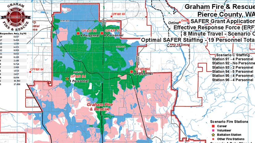
GF&R used its ERF analysis to win a $3.5 million grant from the Staffing for Adequate Fire and Emergency Response (SAFER) program. GF&R provides critical services to a rapidly growing resident population that has increased by more than 45 percent since 1990. This exercise mapped an existing deployment of 15 firefighters and modeled expanded deployments of 17 and 19 personnel. It emphasized creating and managing multiple ArcGIS Pro layouts by using prebuilt ERF polygon and raster layers. For more information on GF&R and the SAFER grant process, see “About Graham Fire & Rescue” in the winter 2019 issue of ArcUser magazine.
The previous exercise modified Pierce County streets and used ArcGIS Network Analyst to model 8-minute travel throughout the GFR service area. The actual staffing criteria included in GFRs grant application was applied to the locations of six GFR stations—five staffed by career firefighters and one staffed by volunteers.
In this tutorial, you will take on the role of a GIS analyst and construct the datasets used in that analysis as well as output maps showing the results of the analysis. This exercise introduces many important ArcGIS Pro concepts and workflows using the Network Analyst and Spatial Analyst extensions for ArcGIS Pro. It re-creates, in ArcGIS Pro, a standard public safety modeling workflow that has been utilized in ArcMap for many years.
Getting Started
- Go to the ArcUser website and download the sample dataset, GFR_SOC.zip. The archive includes a dataset and supporting files for building the model. Extract it to a local machine.
- Go to ArcGIS Online and verify that Network Analyst and Spatial Analyst extensions are available to your ArcGIS Pro license.
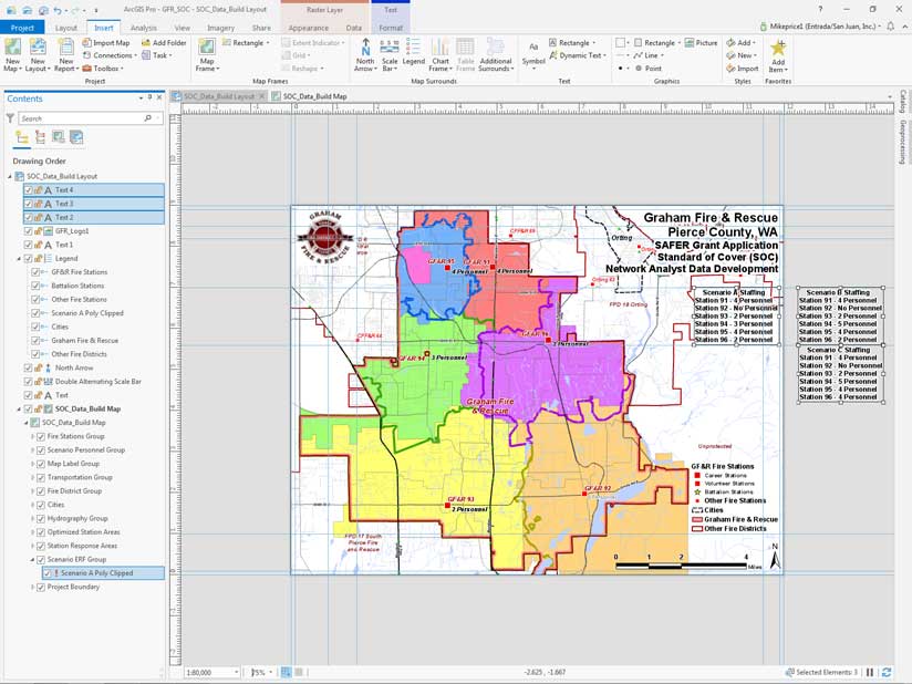
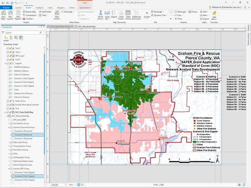
- Start ArcGIS Pro, navigate to where you unzipped GFR_SOC, look in the GFR_SOC folder, and open GFR_SOC.aprx. The map opens in layout view. Open the Contents pane (if necessary). All data layers are visible except Scenario A Poly Clipped, located in the Scenario ERF Group near the bottom. This layer will represent the 8-minute staffing coverage used to create multiple maps. It is a template placeholder for the final ERF output. Do not remove it or try to repair its missing data source.
Notice that this layout includes three text blocks listing staff assignments at stations for three scenarios labeled A, B, and C. Scenario A defines the current 15-person staffing. Scenario B increases staffing by 2 to 17, and Scenario C adds 2 more personnel for a total response force of 19.
Switch to the map view and turn off the Optimized Station Areas and Station Response layers. Use the bookmark GFR SAFER 1:80,000 to navigate to the active project area.
Adding Data and Setting Environments
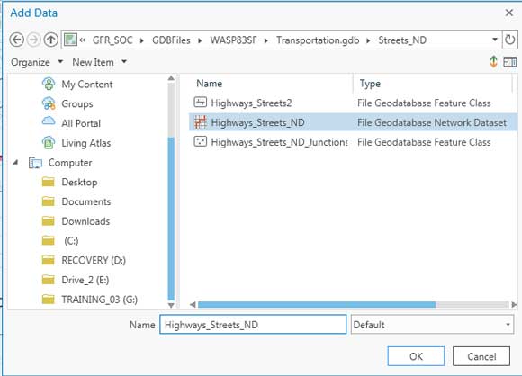
Click Add Data and navigate to GFR_SOC\GDBFiles\WASP83SF and open Transportation.gdb. Open the Streets_ND feature dataset and add only Highways_Streets_ND, the network dataset. Place Highways_Streets_ND in the Transportation Group, drag it to the bottom of the group, and turn it off.
Click Add Data again, navigate to GFR_SOC\GDBFiles\WASP83SF\Cartography.gdb, and open GFR_Clip_Grid. Place this raster at the bottom of the Contents pane and turn it off.
To set Environments, click the Analysis tab, then Environments. Environments are defined in ArcGIS Pro using many of the same modeling rules and parameters used in ArcMap. In the Environments pane, set the Current and Scratch Workspaces to SOC_Model.gdb. Set the Output Coordinate System to GFR_Clip_Grid. Set the Processing Extent and Snap Raster to GFR_Clip_Grid. Finally, set the Cell size to Same as Layer GFR_Clip_Grid. Save the project.
Creating 8-Minute Service Area Polygons
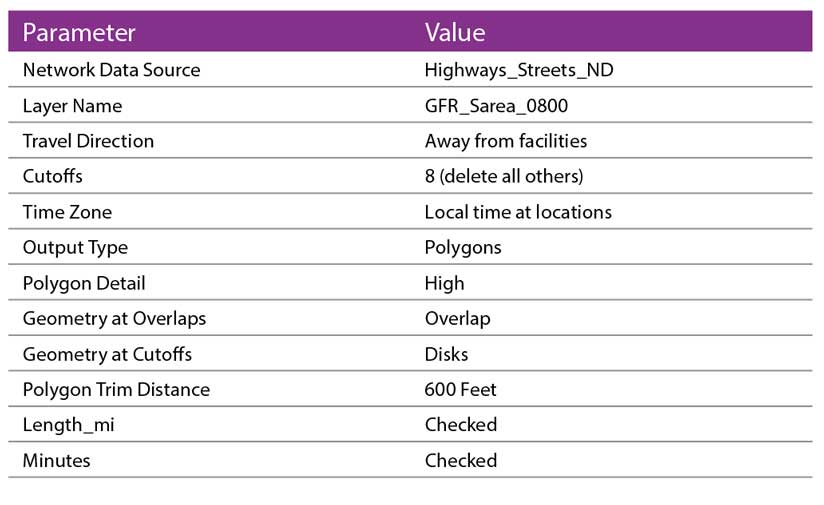
On the Analysis tab, open Tools. In the Geoprocessing pane, click Toolboxes, then choose Network Analyst Tools > Analysis > Make Service Area Analysis Layer tool. Carefully set only the parameters listed in Table 1 and leave defaults for all other parameters. When done, click Run to create the 8-minute Service Area.
Loading Station Locations and Solving Service Areas
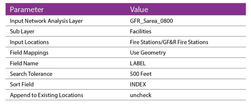
ArcGIS Pro uses a new procedure to load locations into Network Analyst solvers. Add GF&R fire stations to the 8-minute Service Area by choosing Tools > Network Analyst Tools > Analysis > Add Locations tool. In the Add Locations wizard, use Table 2 to set the parameters. Make sure Sort Field is set to INDEX. Make sure Append to Existing Locations is unchecked. When done setting parameters, click Run.
When processing is finished, verify that all six locations have loaded and that the data is sorted by Index. Save the project.
Choose Tools > Network Analyst Tools > Analysis > Solve tool. Set the Input to GFR_Sarea_0800, leave other Solve parameters unchanged, and click Run to generate 8-minute polygons. The polygons are added to the project. Save the project again.
Enhancing and Inspecting 8-Minute Service Area Polygons
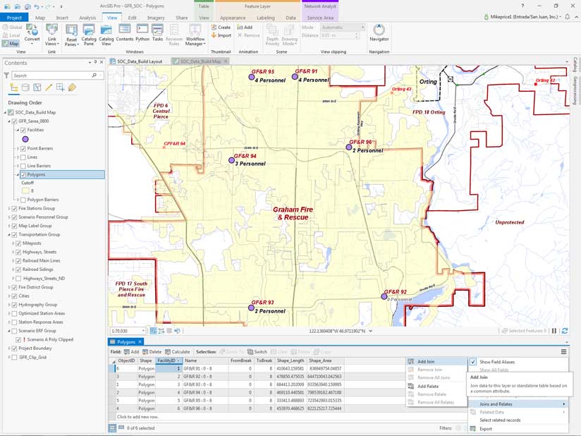
- With SOC_Data_Build Map, go to the Contents pane and under GFR_Sarea_0800, open the Polygons layer attribute table. Dock the table at the bottom of the map frame.
- Sort attributes by FacilityID in ascending order and click three bars in the table’s upper right corner to open its menu. Select Joins and Relates > Add Join.
- In the Add Join pane, set Layer Name to Polygons and Input Join field to FacilityID. This field is not indexed, so it displays a yellow caution symbol, and that is okay. Set Join Table to GF&R Fire Stations. Set Output Join Field to INDEX. Leave Keep All Target Features checked. Click Run. When completed, save the project.
Inspect the joined attributes and sort again on FacilityID. The LABEL field should list in ascending order. Highlight the record for Station 91 and inspect its 8-minute travel area. It is located on an arterial street, so its southern travel capabilities are significant. Note the OBJECTID_1 field—it will soon become very useful. Clear the record selection for Station 91 before moving on.
Exporting Polygons
In the Contents pane, right-click Polygons and select Data > Export Features. In the Copy Features pane, set Input Features to Polygons. For Output Feature Class, save the output in SOC_Model.gdb and name it Sarea_0800_GFR. Click Run. When processing is completed, place GFR_Sarea_0800 near the bottom of the Contents pane, just above GFR_Clip_Grid, and open its attribute table. Turn off GFR_Sarea_0800. Save the project.
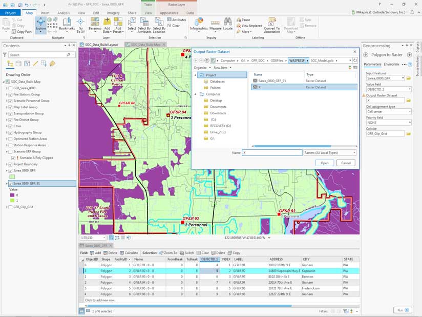
Converting Each Polygon to a Raster and Reclassifying It
- Sort the attribute table for Sarea_0800_GFR by INDEX in ascending order. Find the OBJECTID_1 field. This field will be used to assign values to the initial coverage rasters. Save the project again.
- In the attribute table, select the record for Station 91. In the Geoprocessing pane, use the Search box to find Polygon To Raster. In the Polygon To Raster window
- Set Input Features to Sarea_0800_GFR.
- Set Value Field to OBJECTID_1, NOT OBJECTID. This parameter is very important.
- Set the Output Raster to X and store it in SOC_Model.gdb.
- Verify that Cellsize is managed by GFR_Clip_Grid (which was set in Environments). Click Run to create a temporary raster called x. Since it is temporary, there is no need to move it in the Contents pane. In the Geoprocessing pane, choose Spatial Analyst Tools > Reclass > Reclassify. When the Reclassify pane opens
- Set Input raster to X.
- Reclass field to VALUE.
- Under Reclassification, first row, Value is 4 (which is the value for OBJECTID_1) and set New as 1.
- Under Reclassification, second row, Value is NODATA and set New as 0. It is important reclassify NODATA to zero.
- Name the Output raster Sarea_0800_GFR_91 and store in SOC_Model.gdb.
- Click Run.
The output raster represents the 8-minute travel area for Station 91. Position it just above GFR_Clip_Grid in the Contents pane. Inspect its extent and verify that cells in the coverage area contain a value of 1 and all cells outside the coverage area contain a value of 0.
Remove the x layer and save the project.
For the remaining five station service areas, select each in the attribute table and repeat the steps to convert each service area polygon to a raster and then reclassify the resultant rasters based on the OBJECTID_1 field.
Take your time. Make sure the correct OBJECTID_1 for each record is the Value to reclassify on and 0 is set as New for NODATA. Delete the x layer after reclassifying each station’s service area raster. Name each raster based on the station number. Save the project after creating each raster. Use the Favorites tab on the Geoprocessing pane to quickly locate the Polygon To Raster and Reclassify tools. Close the attribute table for Sarea_0800_GFR when done and turn off all the raster layers you just created.
Creating Effective Response Rasters for Three Scenarios
Environments Mask option, which was not set earlier, will be used to constrain future geoprocessing output to inside the boundary of the GF&R jurisdiction. Click the Analysis tab and click Environments. Set Mask to GFR_SOC/GDBFiles/Cartography.gdb/GFR_Mask_Poly.
Modeling the three separate ERF scenarios will require creating a unique masked ERF raster for each one. To streamline calculations, a text document called ERF_Scenarios_A_B_C.rtf contains the formulas necessary for each calculation. Use your computer’s file manager, not ArcGIS Pro, to navigate to GFR_SOC\Support and open ERF_Scenarios_A_B_C.rtf.
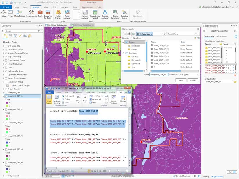
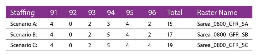
Each formula multiplies individual station travel raster cells by the number of personnel assigned in the scenario. All six raster calculations are summed to model the scenario’s total ERF coverage. The effects on staffing for each scenario is summarized in Table 3 along with the name assigned to each scenario raster. Open ERF_Scenarios_A_B_C.rtf in Microsoft Word or a text editor and make its window accessible when you go back to ArcGIS Pro.
Choose Tools > Spatial Analyst Tools > Map Algebra > Raster Calculator. After activating ERF_Scenarios_A_B_C.rtf, select and copy the Scenario A formula and paste it into the Map Algebra expression window. Copy the output raster’s name from the text file and paste it into the Output raster field. Click Run to solve Scenario A and inspect the results. The raster legend for Scenario A ERF should include a minimum value of 0 and a maximum value of 15. Save the project.
Updating Legends and Data
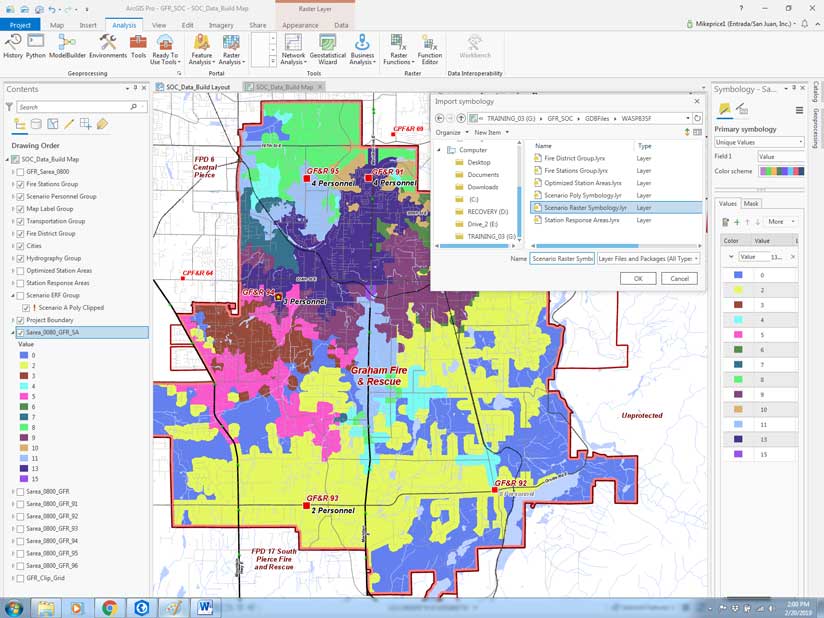
To improve the legend, return to the Contents pane, right-click Sarea_0800_GFR_SA, and select Symbology. Open the Symbology pane’s menu on the upper righthand side, choose Import, select Scenario Raster Symbology.lyr from \GFR_SOC\GFR_SOC\GDBFiles\WASP83SF, and apply the Manual Interval scheme. The Scenario A legend now matches the legends in the previous tutorial. Save the project.
Remember Scenario A Poly Clipped, the undefined feature class in the Contents pane? Update it now to include the Scenario A solution by setting its data source. In the Contents pane, under Scenario ERF Group, right-click Scenario A Poly Clipped and choose Properties > Source and navigate to Sarea_0800_GFR_SA. Click OK and the layer updates. Since this layer now displays raster data, change its name to Scenario A Grid Clipped.
Data in Map View, Legends in Layout View
Click on SOC_Data_Build_Layout to see how the updated legend behaves. Notice that the legend reflects the Scenario A update and shows the correct name and legend style for Scenario A Grid Clipped. Save the project and return to SOC_Data_Build_Map.
Reopen the Raster Calculator in the Geoprocessing pane and model Scenario B ERF using the formula and output name from the ERF_Scenarios_A_B_C.rtf file. Repeat this process for Scenario C.
Check the results to confirm that Sarea_0800_GFR_SB contains 17 or fewer responders and Sarea_0800_GFR_SB includes at most 19 personnel.
ArcGIS Pro Legend Tricks
Wouldn’t it be nice to borrow the Scenario A Grid Clipped legend for Scenarios B and C? In the Scenario ERF Group, right-click Scenario A Grid Clipped and select Copy. Move the cursor to the top of the Contents pane, right-click Scenario ERF Group, and click Paste twice. Rename them Scenario B and Scenario C.
Right-click Scenario B Grid Clipped, open its properties, and change its source to Sarea_0800_GFR_SB. Repeat these steps for Scenario C Grid Clipped. Remove Sarea_0800_GFR_SB and Sarea_0800_GFR_SC from the Contents pane and save the project.
Return to SOC_Data_Build_Layout and locate Scenario A Grid Clipped in the Legend group. Right-click this layer’s legend element and select Save As Default.
Return to the SOC_Data_Build_Layout, left-click and hold Scenario B Grid Clipped, and drag it into Legend. Repeat this process for Scenario B Grid Clipped. Make Scenario B Grid Clipped and Scenario B Personnel (in the Scenario Personnel Group) visible. Turn off the Scenario A Grid and Personnel.
On the pasteboard slightly to the right of the active layout, locate the Scenario B staffing text block. Swap the Scenario A staffing text block with the Scenario B staffing text block. Save the project.
On Your Own
Congratulations. By working this tutorial, you have created enough analytical and mapping materials to support a high-quality SAFER application. Export as a PDF or print Scenarios A, B, and C to share your work with senior staff as you continue—in your hypothetical role as a GIS analyst—to develop your agency’s SAFER application. At this point, you might consider other mapping and modeling options. A great next task would be to convert all three clipped ERF rasters to polygons and calculate their respective coverage areas.
Using polygons, you could compile recent incident points to show how many incidents fall into each responder count cell for all scenarios. You might also compile and rank residents and households for census block centroids by coverage and perhaps classify assessed valuation for protected parcels. You might use these maps and the underlying data to show local officials and residents how they are positively affected by increased levels of protection.
Summary and Acknowledgments
This has been a very interesting tutorial to create and document. It updates a traditional modeling workflow that used ArcView GIS 3.x and has transitioned with rapid changes in software and the world.
Congratulations to Graham Fire & Rescue for receiving a SAFER grant. Thanks again to the GIS data managers in Pierce County, Washington, for providing quality datasets that help represent real-world conditions. Special thanks to Oscar Espinosa, the assistant chief for Graham Fire & Rescue, and his fine staff for their commitment to deploying ArcGIS Pro right out of the box, even though they lacked experience with ArcGIS Desktop. We are learning lots from you, Chief Espinosa.