This exercise continues to explore georeferencing in ArcGIS Pro. The previous exercise, “Georeferencing Drone-Captured Imagery,” in the Winter 2018 issue of ArcUser showed a simple imagery georeferencing workflow that imported an MXD document into ArcGIS Pro. In that exercise, two images were georeferenced by interactively connecting the ground control targets on the raster with vector control points.
This exercise shows how to georeference an image by importing a file containing 29 carefully surveyed ground control points into ArcGIS Pro. The number of well-distributed control points will let you explore the effects of all transformations available in ArcGIS Pro.
The current and previous exercises use drone imagery that was captured in November 2017 during the Canada-United States Enhanced Resiliency Experiment (CAUSE V), which was conducted along the Washington-British Columbia border. The drone imagery used in this exercise is part of a large imagery dataset captured along the Nooksack River and in the town of Everson, Washington, by TacSat Networks of Garden City, Idaho.
For more information about CAUSE V and an overview of georeferencing fundamentals, read “Georeferencing Drone-Captured Imagery” in the Winter 2018 issue of ArcUser magazine.
Getting Started
Begin by downloading and unzipping the sample dataset for this exercise from the ArcUser website (esri.com/arcuser) to a local drive. Note that folders are organized and named to separate the imagery captured by individual drones in specific project areas during the CAUSE V drill. When you are georeferencing your own drone images, consider creating a similar file structure and naming convention.
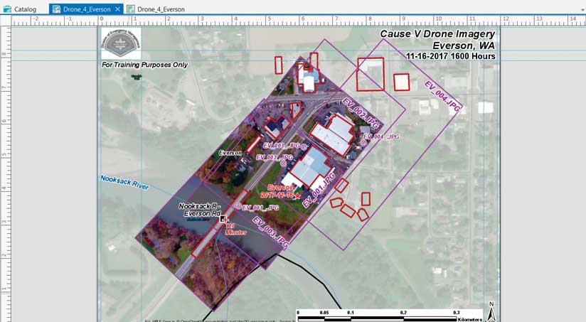
Start ArcGIS Pro, navigate to the Cause_V_controlpts_4/Drone_4_Everson folder, and open the Drone_4_Everson.aprx file. Make sure the map is in layout mode. It should show the two images that were georeferenced in the previous exercise, “Georeferencing Drone-Captured Imagery,” which is available online in the winter 2018 issue of ArcUser.
Carefully study the image outlines shown in the Drone 4 Image Outline layer. In this exercise, ground survey control points that have been saved to a text file will be imported to georeference the EV_004 image.
Adding the EV_004 Image
Switch to the Drone_4_Everson Map frame, click Add Data, and navigate to \CAUSE_V_Drone_4\Imagery\Everson_Images\. Select EV_004.JPG and click OK.
Once the image is loaded, place it immediately below the EV_001 and EV_002 layers in the Contents pane. Reorder image layers so they are in numerical order from 001 to 004. Select all three images, right-click, and add them to a new group and rename it Drone Imagery Group. Turn off all image layers. Save the map.
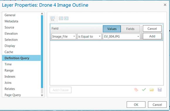
In the Contents pane, right-click Drone 4 Image Outline, select Properties, and open the Definition Query wizard. Create the query Image_File is Equal to EV_004 using either the drop-down selector or the SQL window. Once this definition query is applied, you should see only the image outline for EV_004.
Instead of interactively georeferencing the image as taught in the previous exercise, this exercise will georeference EV_004 by importing control points from a text file located in the Everson_Images folder.
Importing a Control Points File
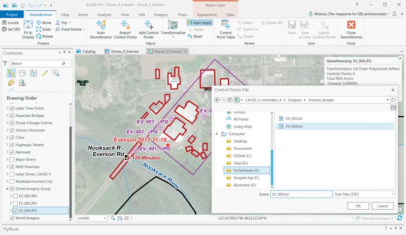
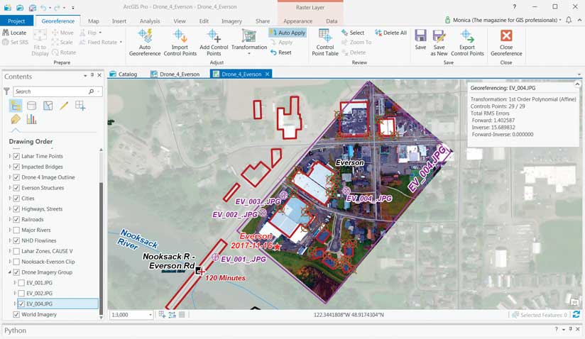
In the Contents pane, turn on the EV_004 image and select it. Click the Imagery tab, click the Georeference button to open the Georeference ribbon, and click Import Control Points. Navigate to \CAUSE_V_Drone_4\Imagery\Everson_Images\ and select EV_004.txt. Click OK. The EV_004 image immediately appears inside the Drone 4 Image Outline.
Study the green control point target symbols in relation to red targets on the image. These symbolized and labeled survey points represent actual locations of red crosses at ground level. The survey control for the image is positioned at ground level on the highway surface and at ground corners—not rooftops—on the image. Because this image was taken at a low elevation, buildings lean away from the center of the image, so only some ground-level corners are visible and rooftop corners are distorted. Save the project.
Testing Transformations
With 29 well-distributed control points for the EV_004 image just imported, all ArcGIS Pro transformation methods can be tried. On the Georeference ribbon, click Control Point Table to open it. This table shows all the imported control points. The default transformation of first-order polynomial (affine) is shown in the drop-down on the table frame. This drop-down will be used to apply the other available transformations. For more on transformations and how they affect georeferencing, read the accompanying article, “Understanding Raster Georeferencing.”
Locate and open the Transformation drop-down and study the available transformation methods. The next section of this exercise explores each transformation method (except zero-order polynomial) by selecting each transformation from this drop-down. Adjust the size of the control points table and zoom out to an extent that enables you to see the EV_004 image and Drone 4 Image Outline to observe the effect of each transformation. You can zoom in to the red and green targets to see how they line up as each transformation is applied.
Do not close the Georeferencing information box, located in the upper right of the map area. Initially it lists measurements for the default transformation, first-order polynomial. This box provides a running count of control points and total RMS errors.
As you apply the different transformations available in ArcGIS Pro, note the effect on measurements listed under total RMS errors. Forward shows errors in the same units as the data frame’s spatial reference. Inverse shows errors in pixel units. Forward-Inverse is a measure of how close accuracy is, measured in pixels. All residuals closer to zero are considered more accurate. RMS error is a good assessment of a transformation’s accuracy, but a low RMS error does not necessarily mean an accurate registration. A transformation may still contain significant errors caused by a poorly entered control point. Study the Georeferencing window to review the RMS error for each transformation.
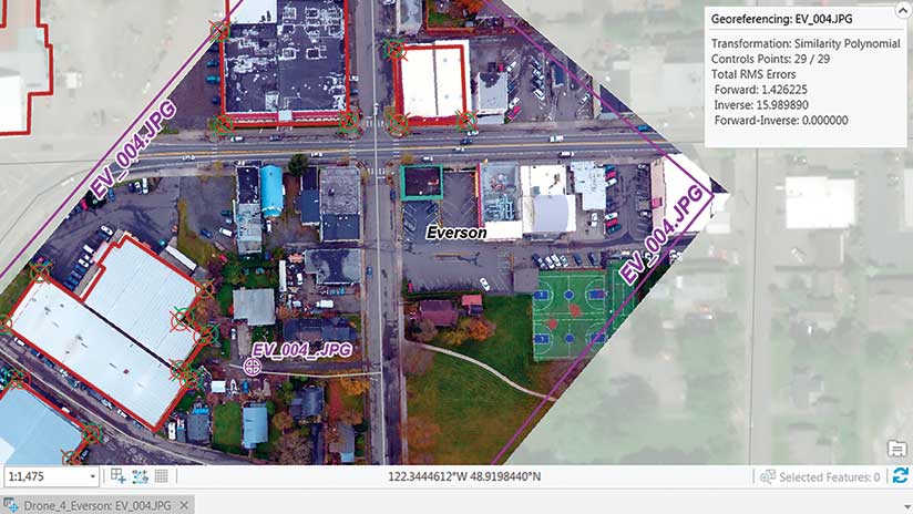
Select Similarity Polynomial
The Similarity Polynomial, a first-order transformation, requires a minimum of three points. It tries to preserve the shape of the original raster, so the overall rectangular shape of EV_004 is preserved but the internal error is typically higher than other polynomial transformations since the preservation of shape is more important than the best fit. The Forward-Inverse Error is zero.
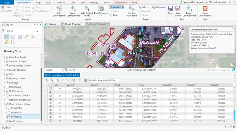
Select the First-Order Transformation (Affine)
Also called an affine transformation, the first-order transformation simply shifts, re-scales, and moves the image. In the early CAD world, this was called “rotate, scale, and move.” If more than three points are used, the error typically increases, although the overall transformation may improve, especially if many accurate points outweigh one or two poorly placed points. Forward-Inverse error is typically zero. The fit within the image frame is slightly rotated.
Select the Second-Order Transformation
This transformation requires six points. It applies a simple quadratic formula (x-squared) to calculate raster cell position. This transformation usually produces a better fit within the image frame and lower Forward and Inverse scores. The image is warped within and near the control points, and the corners match the polygon frame rather well.
Select the Third-Order Transformation
This transformation requires at least 10 points and uses a more complex x-cubed formula. Fit within and around well-placed points is generally very good. However, the raster may be excessively warped along margins. Forward and Inverse scores are typically similar to second order values. Forward-Inverse often appears higher because of excessive edge warp.
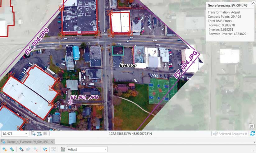
Select the Adjust Transformation
Requiring at least three points, this transformation is optimized for both global least-squares fitting (LSF) and local accuracy. It combines a polynomial transformation with a triangulated irregular network (TIN) interpolation. The Adjust transformation performs a polynomial transformation using two sets of control points and adjusts the control points locally to better match the target control points using a TIN interpolation technique.
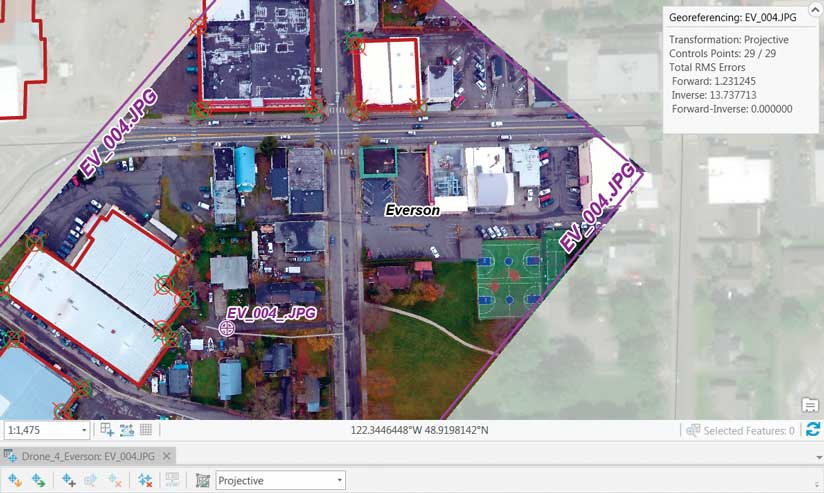
Select the Projective Transformation
The Projective transformation can warp lines so that they remain straight, so lines that were once parallel may not remain parallel. This transformation is especially useful for oblique imagery, scanned maps, and some imagery products such as Landsat and DigitalGlobe. A minimum of four links are required to perform a Projective transformation. When only four links are used, the RMS error will be zero. When more points are used, the RMS error will be slightly above zero.
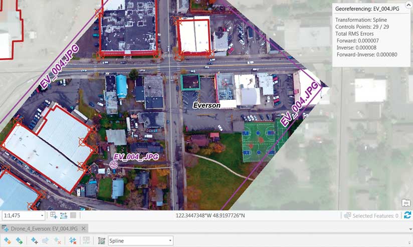
Select the Spline Transformation
Spline transformation is a true rubber sheeting method that is optimized for local but not global accuracy. It is based on a spline function, a piecewise polynomial that maintains continuity and smoothness between adjacent polynomials. Spline transforms the source control points exactly to target control points, so error is minimal. Pixels that are a distance from the control points are not guaranteed to be accurate. This transformation is useful when the control points are important, so those control points must be registered precisely. A spline transformation requires a minimum of 10 points.
Now that you have seen the effect different transformations have on georeferencing, click Close Georeference to complete this exercise and save the project. You may export the map as a PDF or another graphic file as described in the previous exercise using the transformation you like best.
Congratulations, this exercise is complete!
How to Save Georeferencing Information
You can save georeferencing information using one of the options in the Save group on the Georeference ribbon. However, note that these options—Save, Save As New, and Export Control Points—produce different results. The one you choose will depend on what you want to do with the raster.
Save stores the transformation information in separate files using the root name of the image. The type of auxiliary files depends on the original raster format and the selected transformation type. Save does not resample the source raster.
Save As New creates a new raster dataset georeferenced using the map coordinates and spatial reference. You may want to use Save As New if you will be using the raster with software that does not recognize an Esri world file.
Export Control Points creates a file containing control point information. Use it to create or update control information for use with an imported raster in the future, as a backup, or to share control points for the raster with another user.
To summarize, you will most often use Save to update the source raster’s control points and transformation, but use Export Control Points to save the control points to a text file.
Summary
In this exercise, you applied many well-distributed control points that were saved in a text file to georeference an image. You studied the effects of various transformations available in ArcGIS Pro and know how to save georeferencing information with the raster or as control points in a text file for reuse.
Acknowledgments
Again, thanks to the CAUSE V team for giving me the opportunity to participate in this fine exercise. I especially thank Whatcom County Emergency Management and Sheriff’s Office in Washington for all their support. Special thanks to TacSat Network Corporation for providing the drones, operators, and communications.