What if you needed to develop a route in an underwater environment rather than an existing network of streets?
That is the problem that confronted Martha McCauley, a fisheries biologist with EA Engineering, Science, and Technology, Inc., PBC, as part of a fish tracking study of the common carp (Cyprinus carpio) in Manistique Harbor, Michigan.
With funding from the Great Lakes Restoration Initiative, a team of researchers from the US Environmental Protection Agency (EPA) Great Lakes Program Office, the US Army Corps of Engineers (USACE), Michigan Department of Natural Resources (MiDNR), Biohabitats Inc., EA Engineering, and Lotek Wireless conducted a five-month study beginning in June 2016 to track the daily movements of carp in the harbor located at the mouth of the Manistique River. This was part of a study to establish the home range and residency of the carp population occupying the harbor. It would ultimately aid in locating polychlorinated biphenyl (PCB)-contaminated toxic hot spots in the harbor’s bottom sediments.
These hot spots were a result of historical industrial discharges of PCB-contaminated waste into the Manistique River. Although PCBs were banned by the EPA in 1979, the impacts of the contaminated waste on the fish populations that live and forage in the Manistique River can still be seen.
Carp are considered bottom feeders—they consume the organisms that live along the seafloor and therefore are more likely to ingest PCBs that have settled into the sediments. As a result, they are the most heavily contaminated fish in the harbor, which prompted the State of Michigan to issue health advisories against the consumption of carp in the lower river and harbor.
For the purposes of this study, the carp’s PCB contamination level and their direct association with the sediment bed make them useful candidates to help the researchers identify those areas where PCB concentrations in the harbor bottom are high.
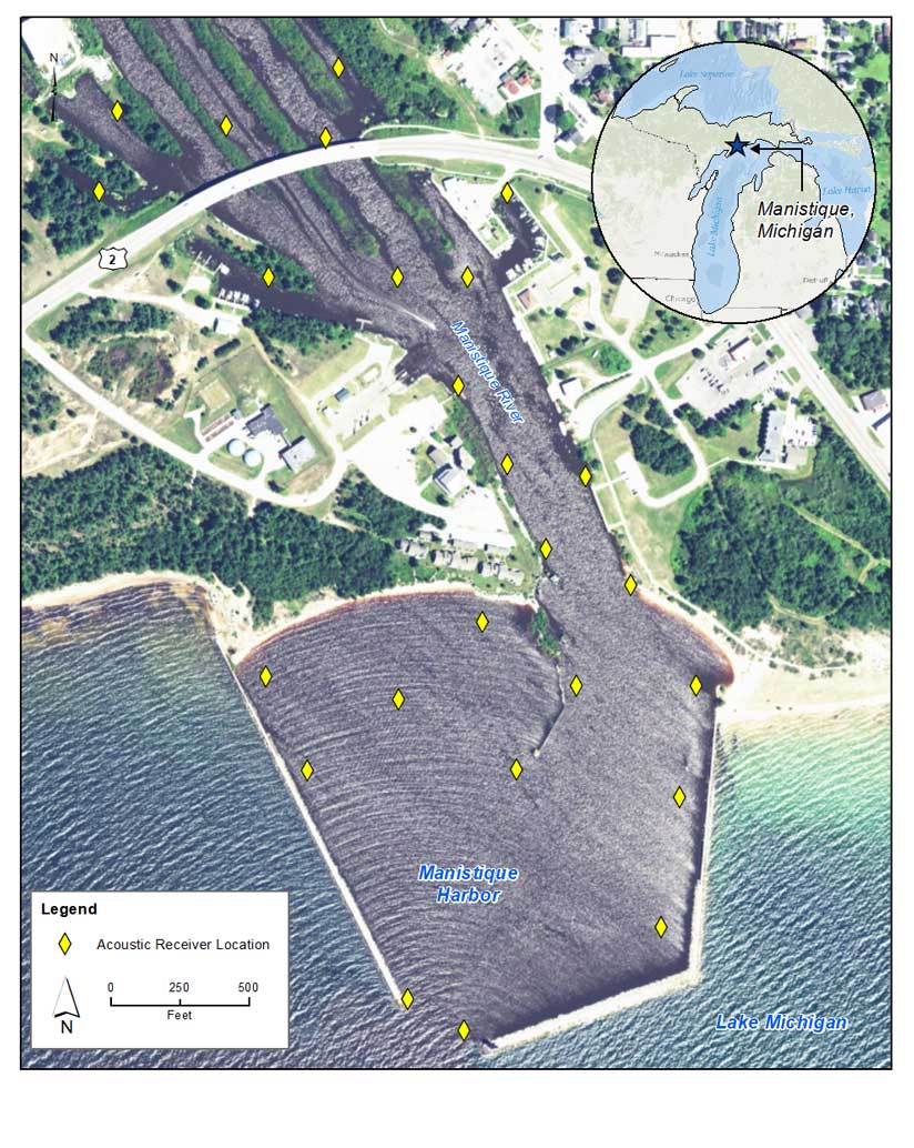
The study tracked the locations of 20 carp over five months to accurately depict their foraging areas. Each fish was implanted with a tiny acoustic transmitter that began emitting a signal once it was released back into the water. The tags produced a signal every five seconds that was picked up by an array of acoustic receivers installed throughout the harbor.
When three or more receivers captured a tag’s signal, the x,y location of the fish was triangulated, time stamped, and recorded with the fish’s tag ID on the receiver’s memory card. To keep up with the large number of data points recorded by the receivers and ensure everything was working correctly, McCauley and her team downloaded receiver data periodically throughout the study.
At the conclusion of the five-month study, more than 5.5 million unique positions had been captured and downloaded, resulting in a detailed but unwieldy dataset. To speed processing time for the ensuing data analysis, McCauley smoothed the dataset in Microsoft Excel by recalculating the points to produce a position every minute as opposed to every five seconds, reducing the number of points to just under a half million positions.
She further increased the dataset’s manageability by exporting each carp’s positional points as a unique dataset based on the carp’s tag ID. This allowed her to work with the data from one fish at a time.
With an average of 23,000 points representing the minute-by-minute position of each fish, McCauley was ready to calculate the swim speed of each carp by using the difference in the x,y position between each consecutive point based on the time stamp. By understanding the fish’s swim speed, she could deduce the behavioral patterns into feeding versus traveling behavior.
However, before she could begin the swim speed calculations, the data points would have to undergo a quality control process to ensure the accuracy of their locations. To view the data in spatial—rather than table—format, McCauley imported the points into ArcMap and plotted them based on each point’s x,y coordinates using universal transverse Mercator (UTM) projection.
The resultant map showed a dense scattering of dots across Manistique Harbor, each dot representing a carp’s location every minute over the course of five months. This allowed McCauley to identify erroneous positions (i.e., positions that fell on land or outside the harbor) and cull them from the dataset. The next step was connecting the points based on their time
stamp. The resultant lines would reveal any gaps in positions that would skew the swim speed calculation.
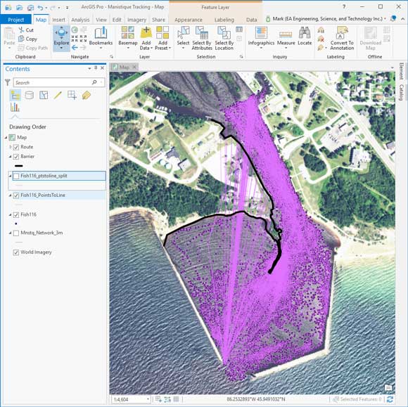
Using the Points To Line tool in ArcToolbox, a massive spider web of lines was generated, covering the harbor and showing the fine-scale movements of an individual carp as it meandered around the harbor during the five-month study. With the lines displayed on an aerial image of the harbor, McCauley discovered where some fish appeared to “jump” back and forth over a large jetty that jutted southward through the center of the harbor.
Carp are not known as a particularly athletic fish, so the line jumps were likely a result of positioning errors that can occur in acoustically challenging areas, such as the deep water adjacent to the rock wall jetty, or exceptionally rough water conditions. These lines would have to be altered to travel around the jetty rather than over it to provide the correct distance between points.
McCauley realized an automated process would be needed to correct the line path of many points. She turned to GIS analyst Mark Dhruv for help. He recognized this as a routing problem. The ArcGIS Network Analyst extension is a great tool for developing customized routes through complex transportation networks, but those are typically street and highway networks.
In this situation, Dhruv employed the ArcGIS Network Analyst extension to revise the segments that crossed the jetty. But before he could begin revising the routes, he needed to create a network layer, and the data would have to be prepped to reroute the “jetty jumpers” as a batch process.
In a typical land-based situation, the Network Analyst extension uses a predefined network, such as streets and highways, to find the shortest or a preferred distance between two points. By inputting a starting and ending point, the tool would create a line segment that adhered to the network layer with any routing variable factored in.
Using this same principle for the watery environment of Manistique Harbor, Dhruv developed a 1-meter by 1-meter grid with the jetty and surrounding landmass factored in. This would serve as the streets or network layer that Network Analyst could use.
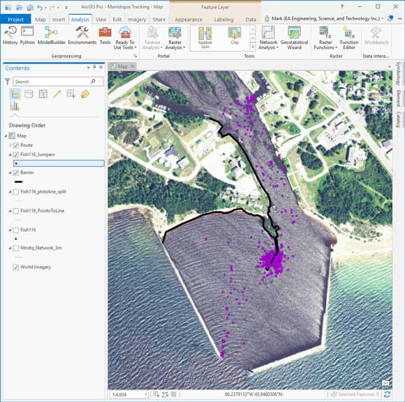
Dhruv prepped the data for batch processing by parsing out the start and end points of the line segments that crossed the jetty. Using the spider web of lines initially created by McCauley, he cut the lines at each vertex to create individual segments. Using the Select By Location tool, he selected the segments that intersected the jetty and exported them as a separate feature.
Using the Feature Vertices To Points tool, an endpoint file for each selected line segment was generated. These points could now be loaded in Network Analyst as stops to create the modified line that would bend around the jetty. This process was repeated for each of the 25 carp.
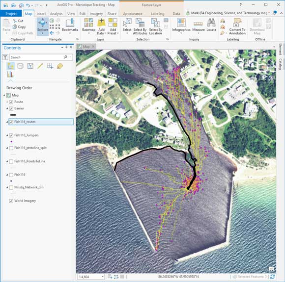
With the data prepped, Dhruv could run the Network Analyst extension. After activating the Network Analyst toolbar, he imported the 1-meter by 1-meter grid as the network dataset and used New Route to load the stops (start and end points of each track) and line barriers (the line layer that outlined the jetty and landmass). After clicking the Solve button, a new line segment was created that ran around the jetty. The length field, revised based on the generated revised segment, now accurately represented the distance traveled by the carp.
Dhruv used a spatial join to merge the revised segment endpoints with the original point data. A simple field calculation replaced the jetty jumper length with the correct length. Now, with her quality control process complete and with a more accurate segment length between point time stamps, McCauley was able to begin her final analysis to identify potential PCB hot spots.
The 1-meter by 1-meter grid was developed to provide the network layer, but additional complexities, such as deeper channels used by fish or known feeding spots, could be added to the project so Network Analyst could be used to create a more realistic network layer.
As shown in this practical application, using Network Analyst to manipulate line segments around barriers isn’t limited to data related to streets and highways. Using Network Analyst in this situation has revealed the extension’s broader capabilities underwater or in any unique environment that requires navigation around barriers.
For more information, contact Mark Dhruv, GIS manager at EA Engineering, Science, and Technology, Inc., PBC, at mdhruv@eaest.com.
Karl Gustavson, Contaminated Sediments Lead, US Environmental Protection Agency, contributed to this article.
About the author