From climate change mitigation and public health improvements to energy independence and grid resilience, solar power adoption delivers a range of climate, public health and economic benefits to the community, utility providers and individual homeowners.

Understanding solar adoption can help to identify trends and inform both private and public campaigns to increase solar adoption in your community. 

Part 1 of this workflow leveraged ready-to-use AI tools and models in ArcGIS Online and ArcGIS Living Atlas to extract building footprints and rooftop solar panels from World Imagery.

Part 2 of this workflow will continue using ArcGIS Online capabilities to calculate solar panel coverage on rooftops, and correlate buildings with demographic data available in Living Atlas. From this additional analysis, insights into solar power adoption within a community can be shared through a dashboard in ArcGIS Online.

Quick links

Use the links below to navigate different sections of this article.

• Terms of Use
• System Requirements
• Analyze Detected Objects
• Correlate Demographic Data
• Visualize Results
• Share Insights

More information

Terms of Use

World Imagery is available for automated information extraction under the following conditions:

• World Imagery layers/services cannot be used as direct input to automated information extraction. Users must export their area of interest to a tile package or hosted tile layer for use as input to information extraction processes.
• Tile packages and tile layers created from World Imagery layers/services are strictly for use within ArcGIS.
• Data and information derived from World Imagery layers, services, and tiles, including but not limited to vector and raster derivatives, are strictly for non-commercial use within ArcGIS.
• Each user is required to have an ArcGIS organizational account.

System Requirements

This workflow requires an ArcGIS organizational account, a minimum of a Professional user type and Publisher role and involves raster analysis in ArcGIS Online which consumes credits. 

Analyze Detected Objects

In Part 1 of this workflow, Feature extraction with AI and World Imagery was executed with two different pre-trained deep learning models available in Living Atlas.  In the Refining Results portion of that workflow, solar panel and building footprint features are stylized, displayed on the source World Imagery tile layer, and saved as a web map.

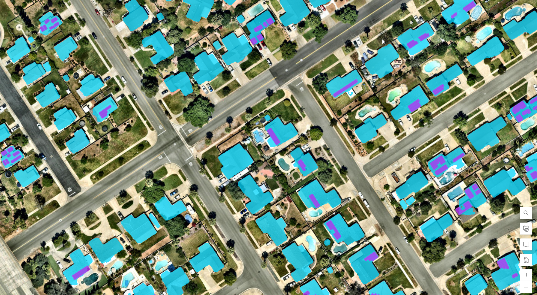
Using the feature layers contained in the Part 1 web map, you can start analyzing solar adoption using built-in capabilities in ArcGIS Online.

Begin by calculating feature area of each detected solar panel, then join these features with the building footprints, to start deriving key metrics about solar panel coverage at the individual building level.

Step 1 – Add a field

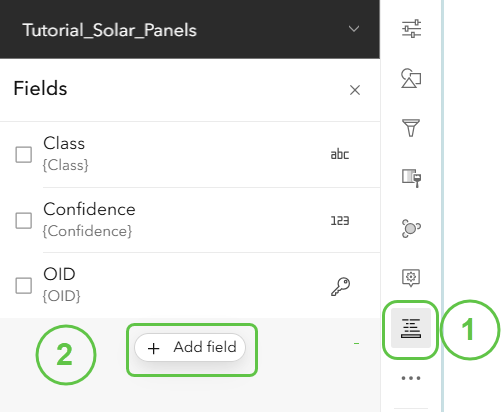
1. With the detected Tutorial_Solar_Panels feature layer selected, click on the toolbar Field button.
2. Select Add field.
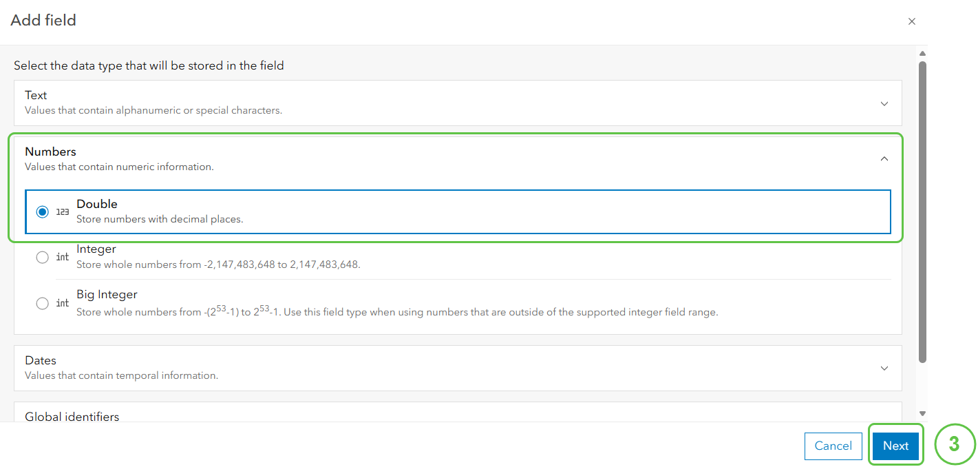
3. When prompted add Numbers field and specify data type of Double before clicking Next.
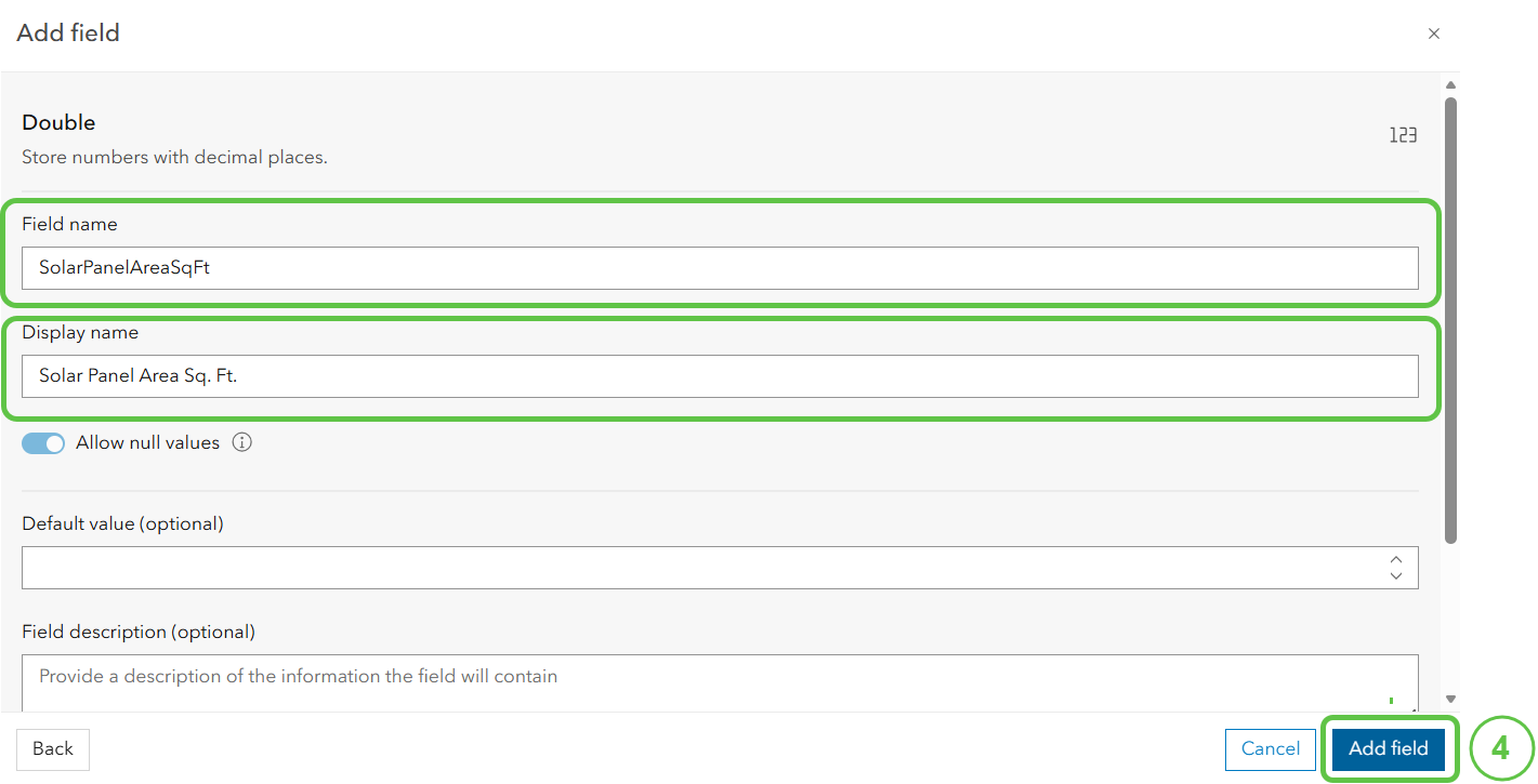
4. Assign the Field name: SolarPanelAreaSqFt and Display name: Solar Panel Area Sq. Ft. then Add Field

Step 2 – Calculate a field

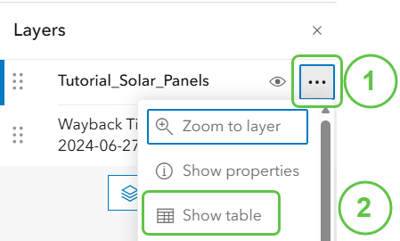
1.  Click on the ellipse … of the Tutorial_Solar_Panels layer to interact with it.
2. Open its table by clicking on Show table.
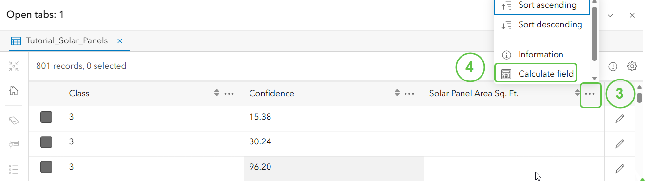
3. In the table, find the Solar Panel Area Sq. Ft. field and click on the ellipse to interact with the field.
4. Select Calculate field.
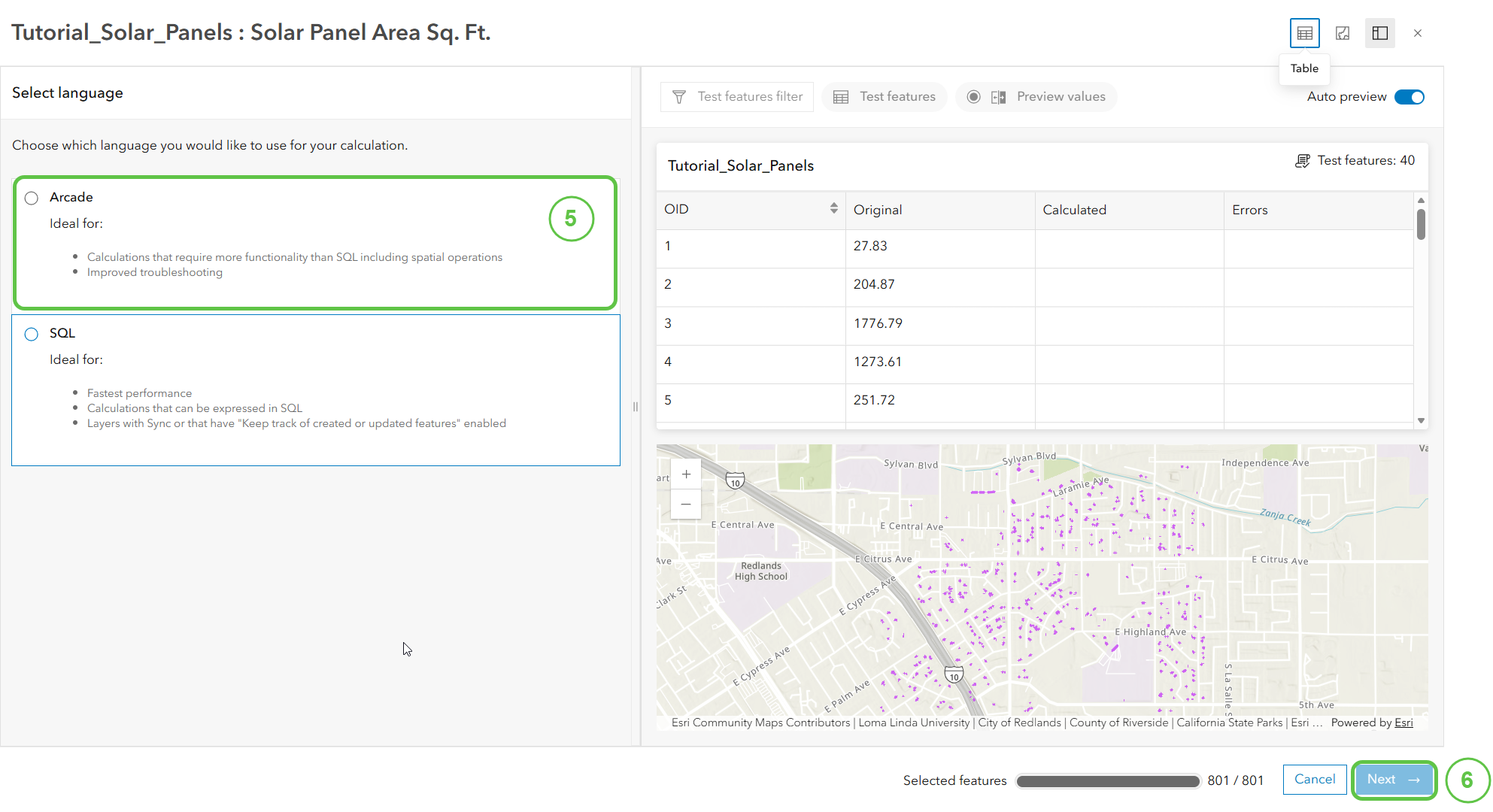
5. When prompted select Arcade language.
6. When prompted to define a filter, select Next to calculate the field for all records.
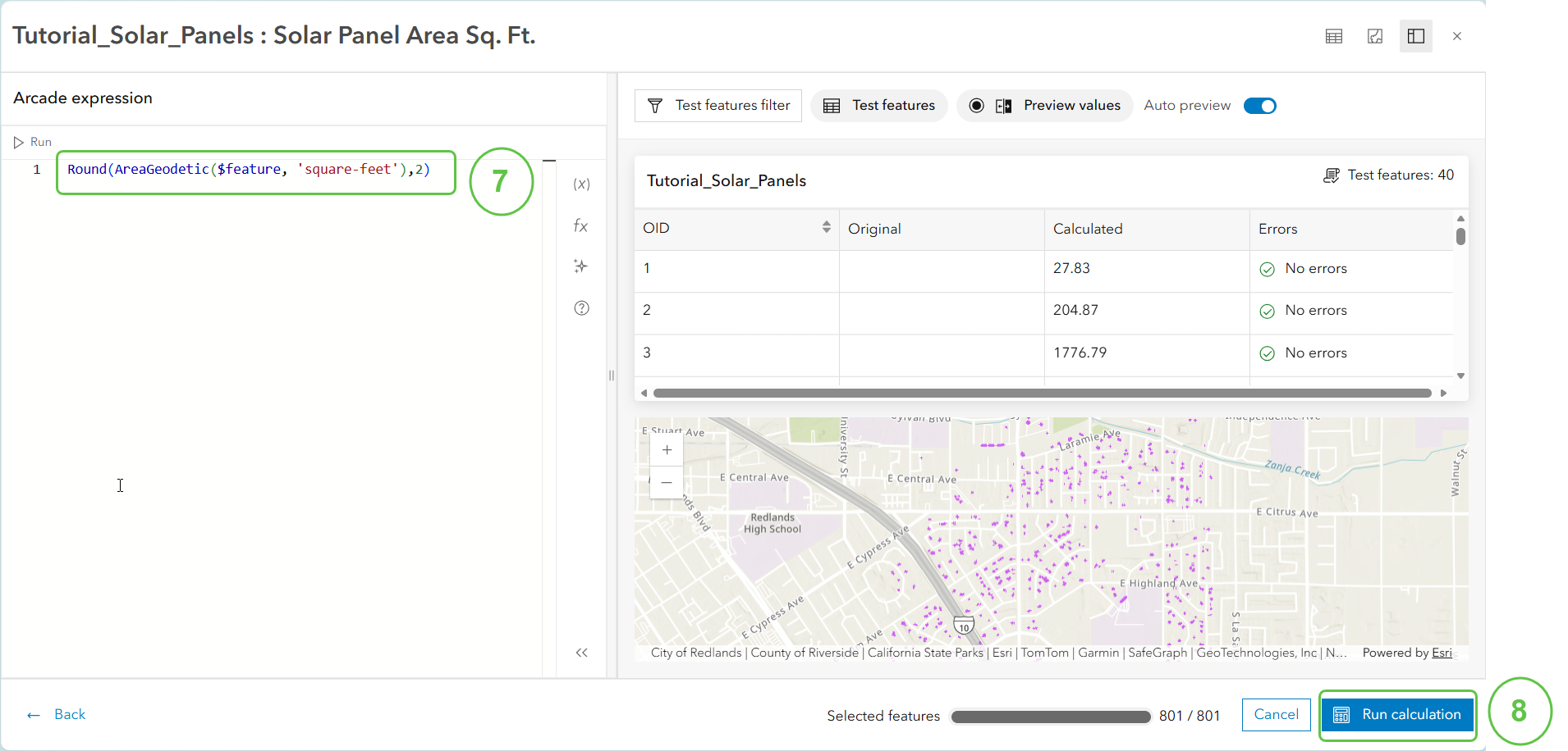
7. Copy and paste this snippet into the Arcade expression window:
   var units = “square feet”; Round(AreaGeodetic($feature, units),2)
8. Run calculation to determine the square footage of each detected solar panel.

Step 3 – Join features

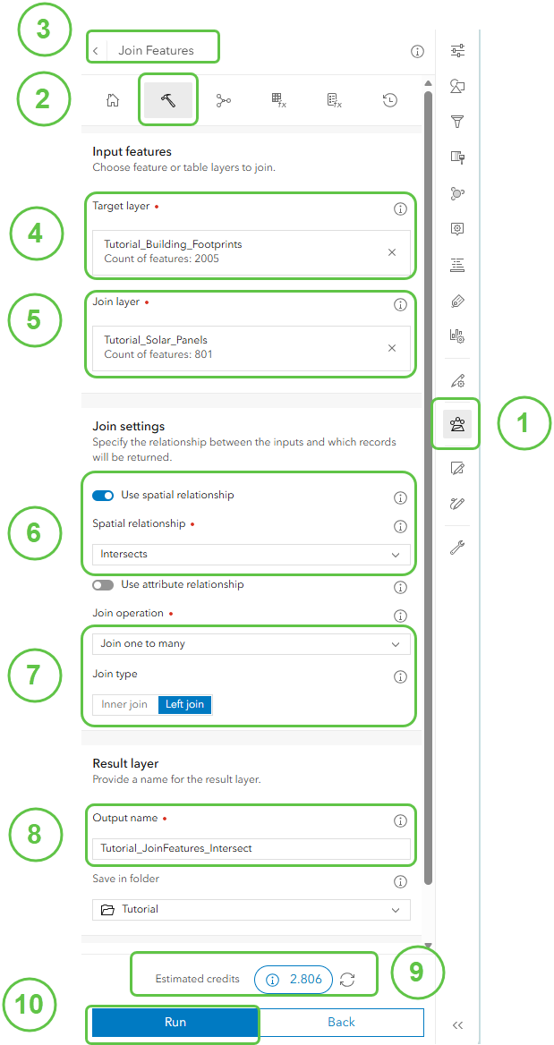
1. Open the Analysis Window.
2. Select Tools.
3. Search for and Select Join Features Tool.
4. Select Tutorial_Building_Footprints as the Target Layer.
5. Select Tutorial_Solar_Panels as the Join Layer.
6. Under Join Settings, select Use spatial relationship with Intersects.
7. Under Join Operation, select Join One to Many with Left Join, to ensure all building footprints are retained.
8. Specify an Output name of Tutorial_JoinFeatures_Intersect.
9. Estimate Credits.
10. Click Run to submit the job.

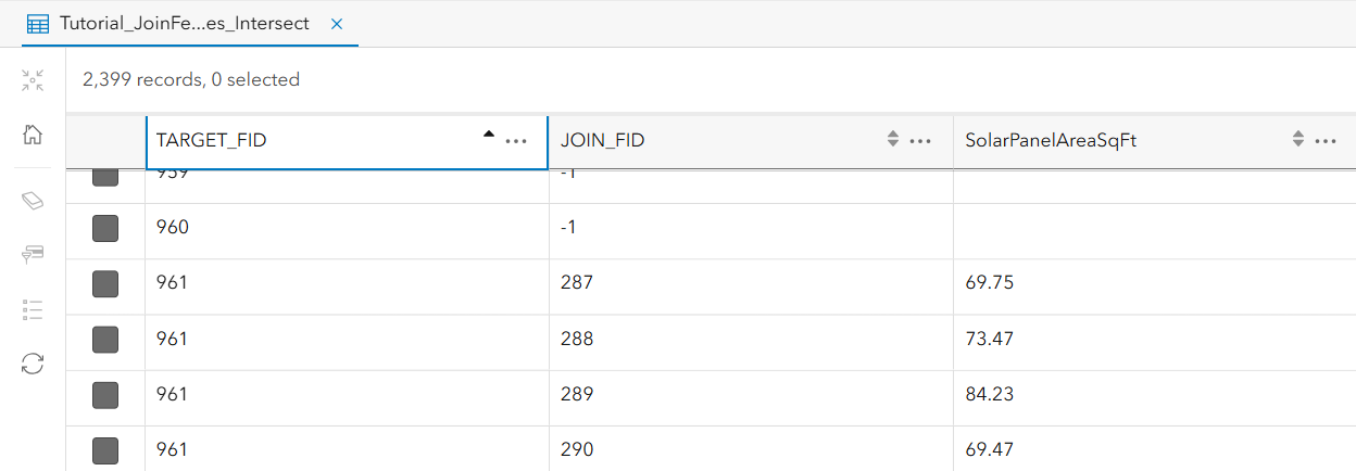
The resulting layer has a record for each building and building/solar panel combination. In the table below you can see that the building TARGET_FID is the same for four records. This means that the building footprint with an original OID of 961 has four solar panels intersecting with its footprint.  The building with an original OID of 960 does not have any solar panels intersecting with it, but because Left Join type was used, this building record was retained.

Step 4 – Dissolve boundaries and summarize area statistics

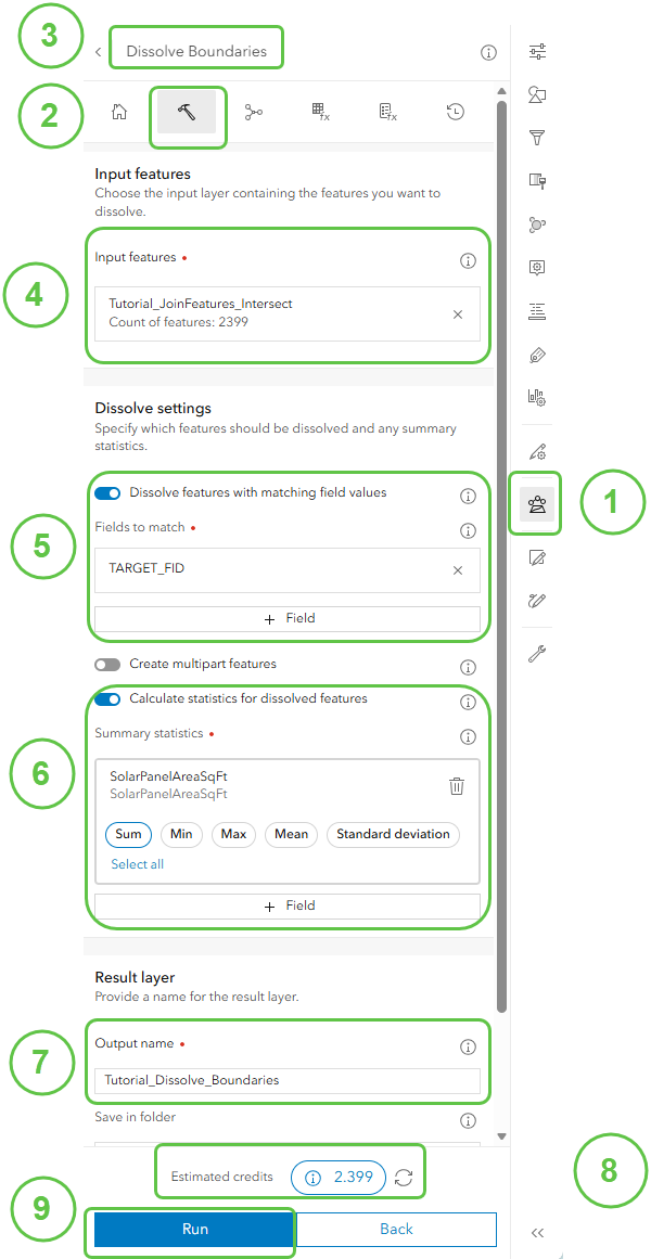
This will create a feature layer where each building has a single record, and an accumulated area for all the solar panels on its roof.

1. Open the Analysis Window.
2. Select Tools.
3. Search for and Select Dissolve Boundaries Tool.
4. Select Tutorial_JoinFeatures_Intersect as the Input Features layer.
5. Dissolve Features based on the Target_FID field.
6. Calculate statistics for the dissolved features and add the field  SolarPanelAreaSqFt and select SUM.
7. Specify an Output name of Tutorial_Dissolve_Boundaries.
8. Estimate Credits.
9. Click Run to submit the job.

Perfom the following steps 5 through 7 on the table of the resulting Tutorial_Dissolve_Boundaries layer.

All three steps involve adding and calculating new fields. References the supporting images from Steps 1 and 2 of this section if you need a refresher on how to access the required tools.

Step 5 – Add a new field and calculate the square footage area for each building.

1. Select Add field
2. When prompted add a Number field and specify data type of Double before clicking Next
3. Assign the Field name: RooftopAreaSqFt  and Display name: Rooftop Area Sq. Ft. then Add Field
4. Calculate the field
5. When prompted select Arcade language.
6. When prompted to define a filter, select Next to calculate the field for all records.
7. Copy and paste this snippet into the Arcade expression window: 
   var units = “square feet”; Round(AreaGeodetic($feature, units),2)
8. Run calculation to determine the square footage of each building footprint

Step 6 – Add a new field and calculate the percentage of rooftop solar for each building.

1. Select Add field.
2. When prompted add a Number field and specify data type of Double before clicking Next.
3. Assign the Field name Rooftop_Solar_Percentage with the Display name Rooftop Solar Percentage and Add Field
4. Calculate the field
5. When prompted select Arcade language.
6. When prompted to define a filter, select Next to calculate the field for all records.
7. Copy and paste this snippet into the Arcade expression window: Round(($feature.SUM_SolarPanelAreaSqFt/$feature.AnalysisArea) *100,2)
8. Run calculation to determine the percentage of rooftop area covered by solar panels.

1. Select Add field.
2. When prompted add a Text field.
3. Assign the Field name: Solar_Status and Display name: Solar Status then Add Field
4. Calculate the field
5. When prompted select Arcade language.
6. When prompted to define a filter, select Next to calculate the field for all records.
7. Copy and paste this snippet into the Arcade expression window: var solarArea = $feature.SUM_SolarPanelAreaSqFt;
   if (solarArea > 0) {

       return “Solar Power”;

   } else {

       return “No Solar”;

   }
8. Run calculation to determine the solar status of buildings. 

Correlate Demographic Data

Household income can correlate with rooftop solar adoption. American Community Survey (ACS) household median income data is available in Living Atlas. Joining this demographic data with the enhanced building layer, will enable visualization of trends around adoption for the community as they relate to household median income.

Step 1 – Add demographic data to the map

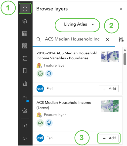
1.  Click on the plus + icon to add a new layer to the map.
2.  Search Living Atlas for ACS median household income data.
3.  Add the latest ACS data for Median Household Income layer.

Step 2 – Explore the Demographic Data

1. Click on the layer ACS Median Household Income to expand the dataset.
2. Observe that the ACS data has layers at the State, County and Tract level.
3.  Notice that at the Tract level, the area where building and solar features were extracted covers 3 distinct Median Household Income Tracts.

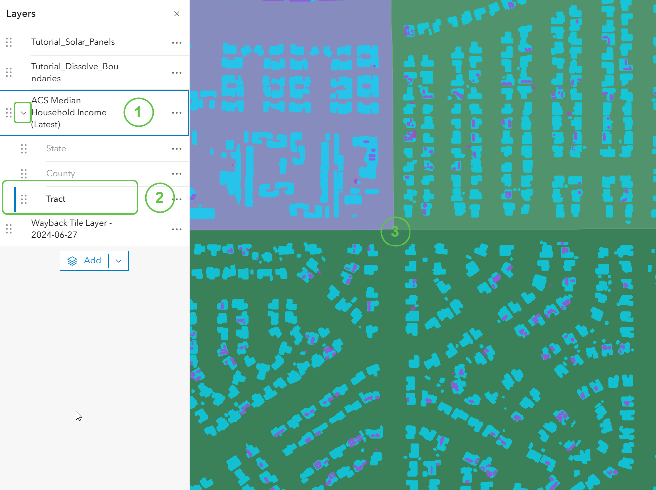
With the ACS Median Income Tract data added to your map, you can Join Features to associate the median income tract information with individual building footprints.

Step 3 – Join Features

1. Open the Analysis Window
2. Select Tools
3. Search for and Select Join Features Tool
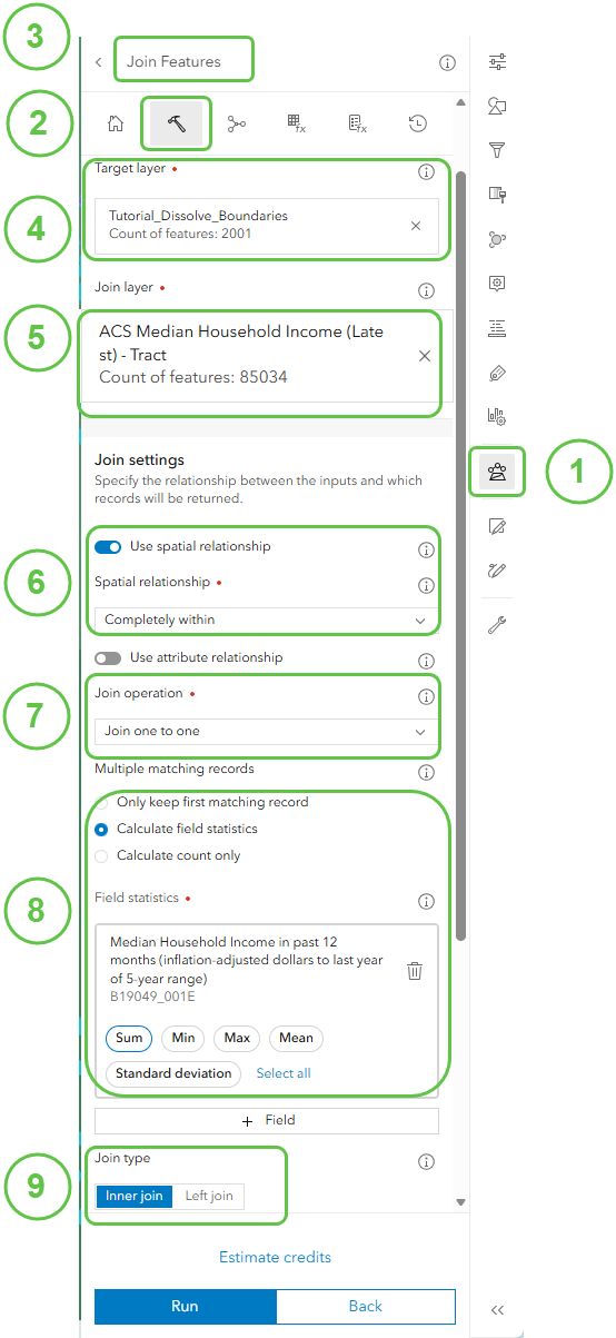
4. Select Tutorial_Dissolve Boundaries as the Target Layer
5. Select ACS Median Household Income Tract Layer as the Join Layer
6. Under Join operation, Use spatial relationship of Completely Within
7. Under Join Operation, select One to One
8. Calculate field statistics using the Median Household Income in past year (B19049_001E)
9. Select a Join type of Inner Join
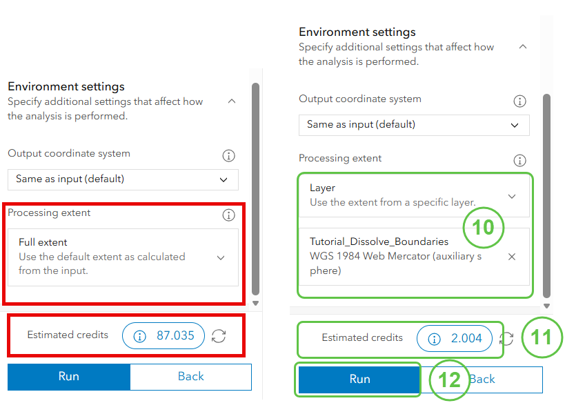
10. In Environment Settings set Processing extent to Layer, add Tutorial_Dissolve Boundaries layer
11. Estimate Credits
12. Run to submit the job

 

Note:  The ASC Median Income Item is nationwide data, so be sure to limit the extents of your output to the Tutorial_Dissolve_Boundaries layer, and not the Full Extents of the input data. One warning sign is if the estimated credits for this join are higher than expected.

The resulting layer will contain the following fields:

• Rooftop Area Sq. Ft.
• Solar Panel Area Sq. Ft.
• Rooftop Solar Area Percentage
• Solar Status
• A new field (SUM_B19049_001E) that associates each building with the Median Household Income associated with the census tract that the building is contained in.

Step 4 – Add a new field for Median Household Income that is more descriptive

Step 1 – Use the Solar Status field to symbolize the building layer.

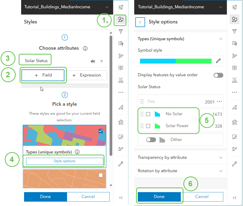
1. Edit Symbology, with the Tutorial_Buildings_MedianIncome layer selected
2. Choose an attribute field to style based on.
3. Select Solar Status field
4. Select Style Options
5. Click on Solar Status legend items to customize Names and Colors
6. Run to execute the symbology changes.
7. Save the web map as Solar Power Adoption

Once a web map is configured and saved, you can use it as a foundation for building a dashboard, to visualize patterns related to solar adoption in the community.

Share Insights

Creation of a web map and application move us from feature extraction and data preparation into visualization and storytelling within ArcGIS Online.

The following web map and dashboard help summarize patterns and trends—making it easier to explore and communicate insights about solar adoption in a community. It can help users answer questions such as:

Is solar power adoption growing in the community?

Is there a correlation between solar power adoption and median household income?

Are existing solar powered homes increasing their capacity?

What percentage of growth is related to new solar adoption?

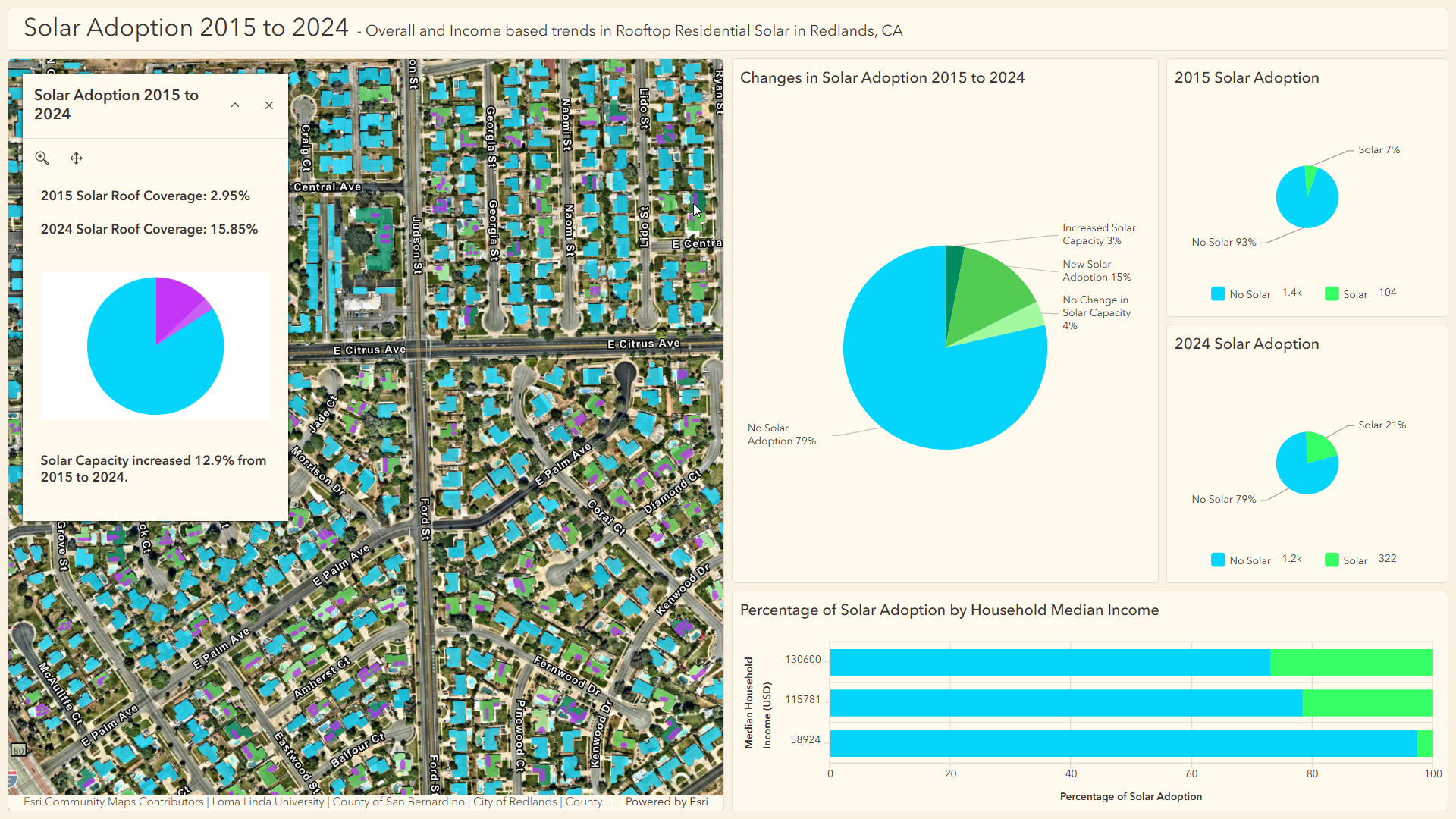
For creation of the above dashboard, historical context was added by repeating Part 1: Feature Extraction with AI and World Imagery using the 2016-02-04 release of the World Imagery basemap, which contains Nearmap aerial imagery captured on 2015-11-21.  Explore this version of World Imagery using the Wayback app.

The Analyze Detected Objects portion of this Part 2 workflow was repeated using the 2015 building and solar panel data, then combined with the 2024 results in a web map. Symbology highlights solar adoption over time, while a custom Arcade pop-up helps illustrate changes in solar coverage at the individual building level.

The resulting dashboard illustrates solar adoption correlation to median household income, and changes in solar adoption in the community over the nine-year period.

More Information

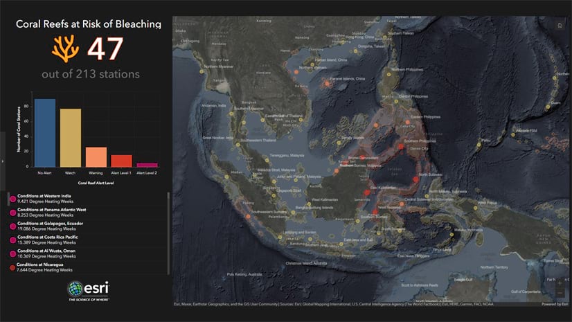
ArcGIS Dashboard is a web-based application used to visualize the data represented in the source web map. In addition to displaying the web map, several components can be added to the dashboard to help focus users on insights extracted directly from the data. If you are new to dashboard, review this Esri Blog Article on how to Create your first dashboard using ArcGIS Dashboards.

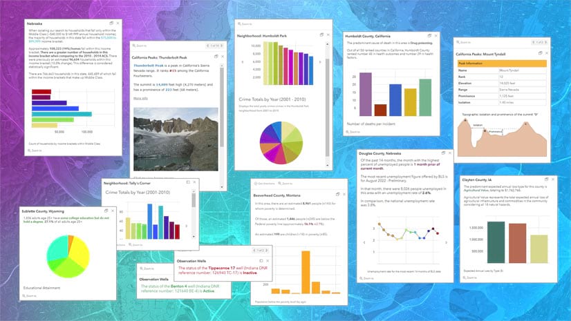
In the Web Map the buildings layer is enabled with a custom pop-up that allows users to visualize solar coverage of individual buildings and see how solar adoption has changed over time.  For more details on how to create meaningful pop-ups, check out Pop-ups: the essentials blog.