Oil spills from ships, tanker accidents, and offshore platforms have been a global concern for marine ecosystems, coastal communities, and fisheries. Early identification of oil spills is essential for guiding effective response efforts, minimizing environmental damage, and reducing economic losses.
The Taylor Energy oil spill, which continued from 2004 to 2019, is the longest-running oil spill in United States history. The spill was caused by the destruction of the Taylor Energy platform about 15 kilometers off the shore of South Pass, Louisiana, during Hurricane Ivan. It resulted in thin layers of floating oil, called oil slicks, and significantly contributed to oil pollution in the region.
As an image analyst working for an environmental agency, your objective is to efficiently extract an oil slick from a Synthetic Aperture Radar (SAR) satellite image and show the extent of the oil pollution. Manual oil slick detection in satellite imagery can be costly, time consuming, and relies upon an experienced analyst to correctly identify the targets. In this blog tutorial, you’ll detect the oil slick in a more automated fashion using a deep learning model. Over the course of approximately 50 minutes, you’ll create a web map containing Sentinel-1 RTC dynamic imagery available through ArcGIS Living Atlas of the World, preprocess your imagery of interest, and apply a pretrained deep learning model to it to extract the oil slick.
Table of Contents
- System Requirements
- Create a web map with Sentinel-1 RTC imagery
- Apply dynamic imagery capabilities
- Apply a pretrained deep learning model

System Requirements
- An ArcGIS Online organizational account with credits*
- A minimum of a Professional User Type with a Publisher role.
- Imagery layers optimized for analysis enabled for your organization**
*This blog tutorial consumes a total of approximately 2 credits. The number of credits will vary depending on the temporal and geographic extent.
**Analysis-optimized Living Atlas imagery layers provide scalability for larger and more diverse workflows. This capability must be enabled to avoid size constraints and allow the analysis to scale appropriately. See ArcGIS Living Atlas ready-to-use imagery layers for analysis for more information, including how to enable imagery layers optimized for analysis.
Create a web map with Sentinel-1 RTC imagery
Satellites with SAR sensors produce images based on radar technology. One of SAR’s strengths is that it can create clear images in the daytime and nighttime alike and regardless of the presence of clouds or rain.
SAR imagery has been widely used for marine oil spill detection because of its high-resolution, large-scale, all-day, all-weather imaging capabilities. Oil slicks appear as dark targets in SAR images (see Alpers and Espedal). To detect an oil slick at the Taylor site, you’ll use Sentinel-1 RTC dynamic imagery available in ArcGIS Living Atlas. You’ll open the dynamic imagery layer in ArcGIS Online and save it in a web map.
Create a folder
First, you’ll create a folder on ArcGIS Online to contain the data layers and web maps resulting from this workflow.
- Sign in to your ArcGIS organizational account.
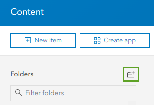
- On the ribbon, click the Content tab.

- Next to Folders, click the Create new folder button.
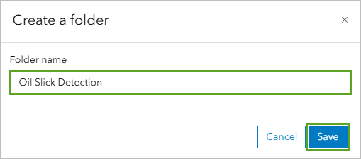
- For Folder Name, type “Oil Slick Detection” and click Save.
The folder is created and becomes your current folder. You’ll use this folder to store all your blog tutorial-related items.
Explore Sentinel-1 RTC dynamic imagery
You’ll look for the Sentinel-1 RTC dynamic imagery layer in ArcGIS Living Atlas.
- In a new web browser window, open ArcGIS Living Atlas of the World.
The home page includes a search bar you can use to search for contents by keywords.
- In the search bar, type “Sentinel-1 RTC” and press Enter.
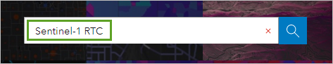
The Sentinel-1 RTC item appears in the search results.
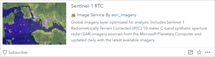
- Point to the Sentinel-1 RTC thumbnail and click View item details.
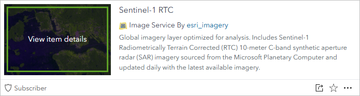
The Sentinel-1 RTC layer’s item details page appears.
- Review the content of the page.
Sentinel-1 RTC provides a 10-meter C-band SAR dynamic imagery that has undergone radiometric terrain correction. This analysis-ready imagery is derived from Sentinel-1 Ground Range Detected (GRD) Level-1 products produced by the European Space Agency.
Create a web map
You’re now ready to open the Sentinel-1 RTC dynamic imagery layer in ArcGIS Online and create a web map.
- On the Sentinel-1 RTC item details page, choose Open in Map Viewer.
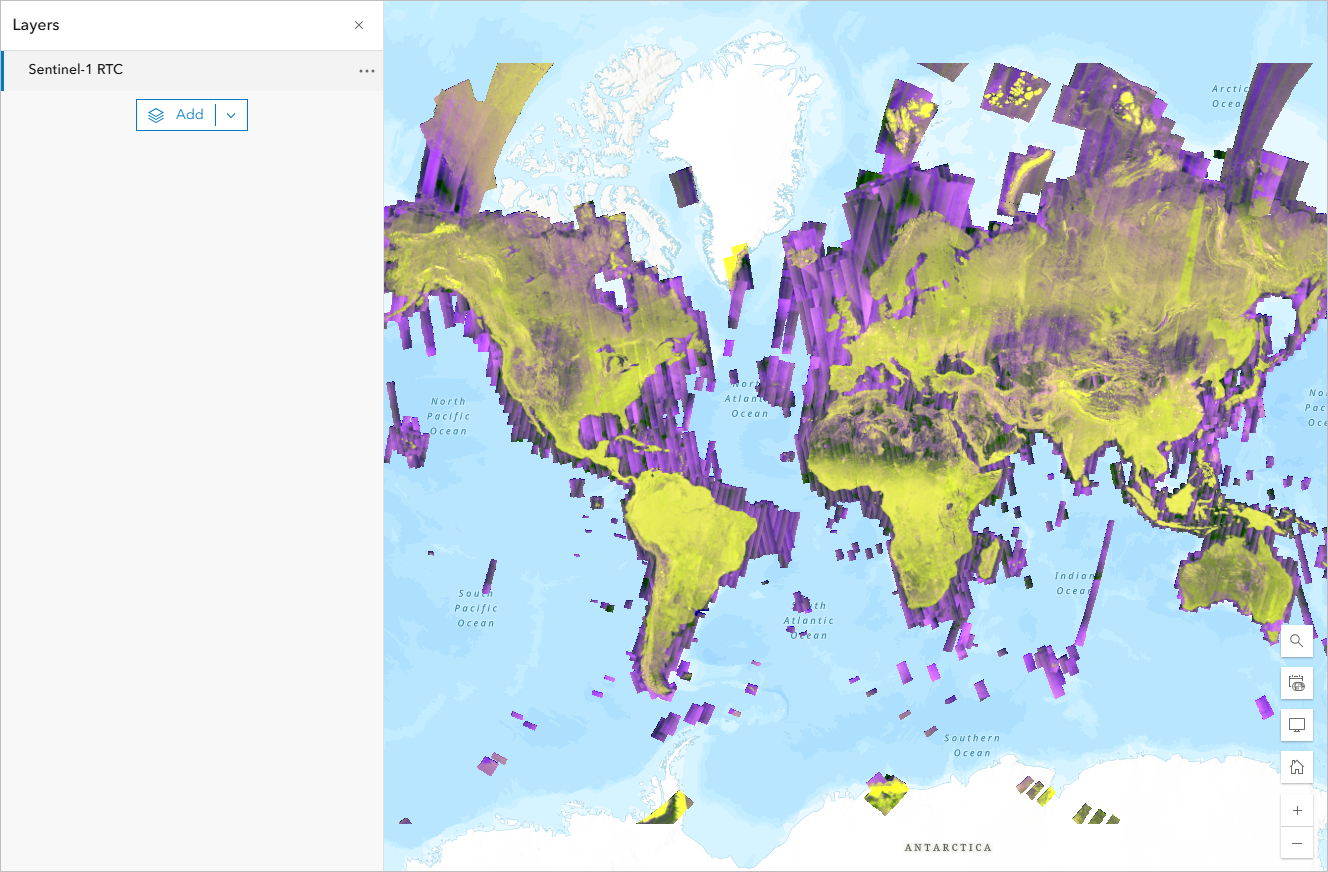
The Sentinel-1 RTC layer appears in Map Viewer, displayed over the default Topographic basemap.
- If necessary, on the top ribbon, sign in to your ArcGIS organizational account.
You’ll save the map to the Oil Slick Detection folder you created earlier.
- On the left ribbon, click Save and open and choose Save as.
- In the Save map window, enter the following information:
- For Title, type “Taylor Oil Slick Site”.
- For Folder, select your Oil Slick Detection folder.
- For Tags, type “Sentinel-1 RTC”, “Taylor site”, and “Oil slick” and press Enter after each tag.
- For Summary, type “Map of the Taylor oil slick site”, or a more detailed summary of your choice.
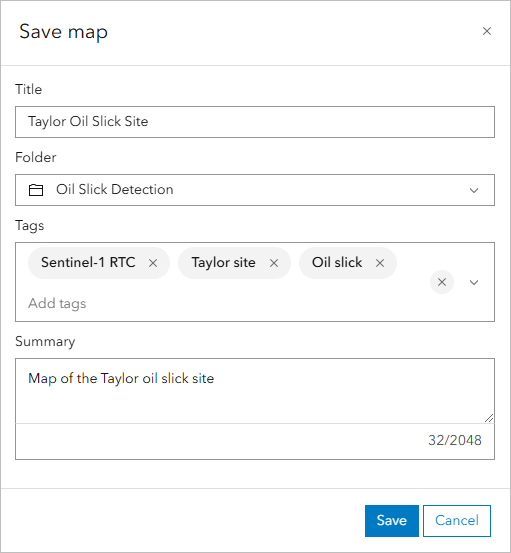
- Click Save.
You’ve created a web map that contains the Sentinel-1 RTC dynamic imagery layer.
Apply dynamic imagery capabilities
Next, you’ll continue preparing your map. The Sentinel-1 RTC dynamic imagery layer contains a growing archive of Sentinel-1 imagery (from 2014 to present) all over the world. You’ll select a single image from the archive for your analysis. That image should cover the Taylor site and have been captured around your date of interest (April 2018). You’ll also apply on-the-fly preprocessing to this image to obtain the appropriate rendering for your workflow.
Add a lease blocks layer
The map you created shows the Sentinel-1 RTC data for the entire world. You need to focus the map to your area of interest (AOI), which is the Taylor site. You’ll use a feature layer outlining the USA Outer Continental Shelf Lease Blocks to do that. These Lease Blocks are legal subdivisions of United States submerged lands, subsoil, and seabed. The Taylor site is in the Mississippi Canyon lease block 20 (MC20).
First, you’ll add the USA Outer Continental Shelf Lease Blocks layer from ArcGIS Living Atlas to your map.
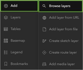
- In your Taylor Oil Slick Site web map, on the left ribbon, click the Add button and choose Browse layers.
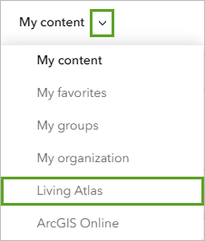
- On the Browse layers item details page, next to My content, click the drop-down arrow and choose Living Atlas.
- In the search bar, type “USA Lease Blocks” and press Enter.
- In the result list, identify the USA Lease Blocks layer owned by Esri.
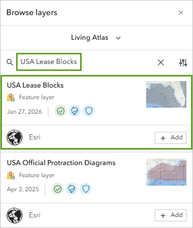
- Click the USA Lease Blocks layer name.
The item details pane for the layer appears.
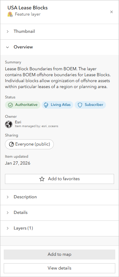
You can read more details about the layer in the pane.
- In the USA Lease Blocks details pane, click Add to map.

The map updates to show the new layer, and automatically zooms to the layer extent.
- Close the item details pane.
- On the left ribbon, click Layers.

In the Layers pane, the USA Lease Blocks layer is now listed.
Select a lease block
Next, you’ll select Mississippi Canyon lease block 20 (MC20) to center the map on the Taylor site. This was the location of the Taylor Energy platform from which the oil spill originated. You’ll use a filter to display only the MC20 lease block in the USA Lease Blocks layer.
- In the Layers pane, confirm that the USA Lease Blocks layer is selected. Click the Filter button on the right ribbon.

The Filter window appears.
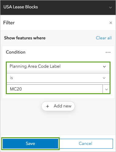
- In the Filter window, click Add new, use the fields to create the condition Planning Area Code Label is MC20, and click Save.
- In the Layers pane, point to the USA Lease Blocks layer, click Options, and choose Zoom to layer.
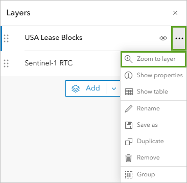
The map updates to show only the MC20 lease block in the USA Lease Blocks layer and zooms to it. You’ll change the style of the layer to make it more visible.
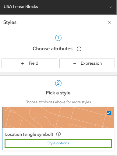
- In the Layers pane, confirm that the USA Lease Blocks layer is selected. Click the Styles button on the right ribbon.

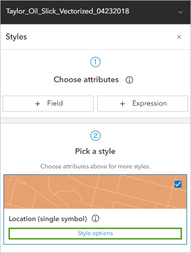
- In the Styles pane, under Pick a style, for Location (single symbol), click Style options.
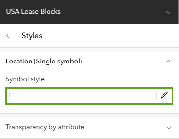
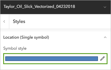
- Under Location (Single symbol), click Symbol style.
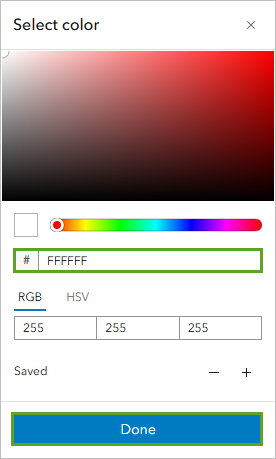
- In the Symbol style window that appears, click the Outline color tab and in the color picker, choose the white color (#FFFFFF). Click Done.
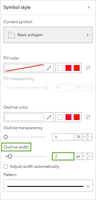
- In the Symbol style window, for Outline width, type 2.
- In the Styles pane, click Done and click Done.
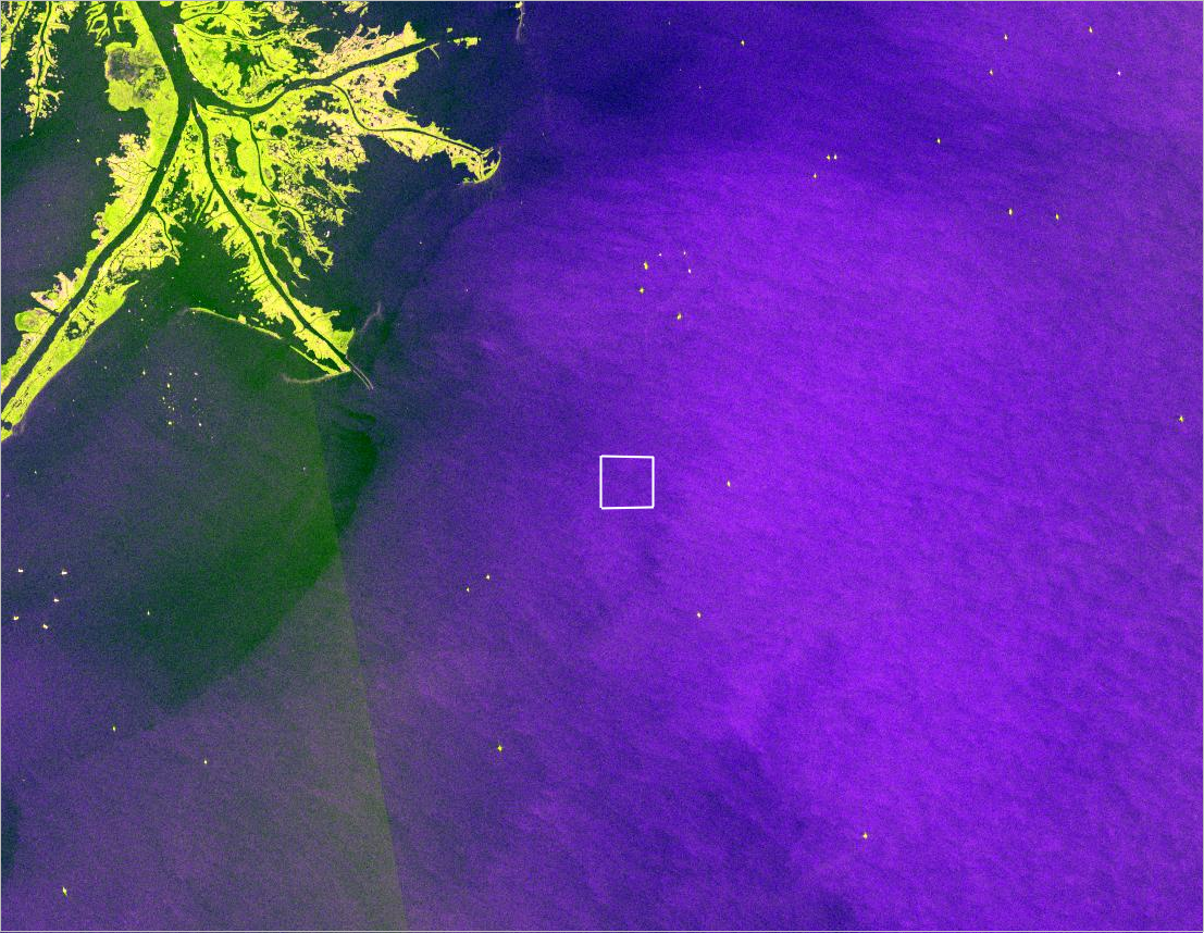
The map now displays the MC20 lease block in white.
- Click the Zoom Out button four times.

You can now clearly see the MC20 lease block where the former Taylor Energy platform was located.
Select an image of the Taylor oil slick
The Taylor Energy oil spill began in 2004 and continued until its containment in 2019. The Sentinel-1 RTC dynamic imagery layer provides images of the Taylor site from 2015 onwards. For the purpose of this blog tutorial, you want to find an image that was captured in April 2018.
- On the left ribbon, click Map properties.

- In the Map properties pane, under Time, for Time zone, select Data’s time zone (no adjustments). This displays the date and time based on the time zone that has been defined for the Sentinel-1 RTC layer.
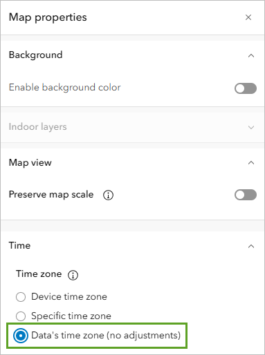
Close the Map properties pane.
- In the Layers pane, confirm that the Sentinel-1 RTC layer is selected. Then click the Image collection explorer button on the right ribbon.
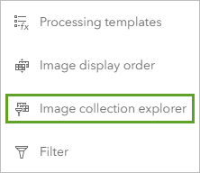
The Image collection explorer pane appears.
This tool will list all available images that intersect your current map extent. By default, this tool lists images available in your layer according to “best” criteria. You need to change it to AcquisitionDate to sort by the date when the images were captured.
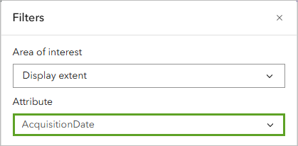
- In the Image collection explorer pane, click the Filters button.
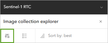
- In the Filters window, Under Attribute, select AcquisitionDate.
Next, you’ll change the range mode.
- Drag the handles to span from January 1, 2018, to December 30, 2018.
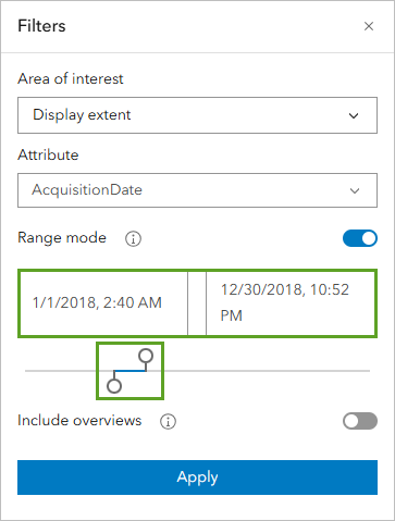
Defining this time range will allow you to quickly narrow down the list of relevant images and identify your image of interest.
- Click Apply and close Filters window.
- Under Image collection explorer, scroll down and find the image where AcquisitionDate is April 23, 2018.
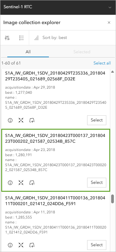
Note: Clicking “Select” for an item in the list will provide a preview of that image. You can view the image in full and visually inspect it to decide whether the image is relevant for your purposes.
- Add the image for April 23, 2018 by clicking on Add image to map icon.
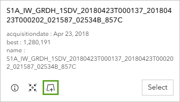
In the Layers pane, a new imagery layer named Sentinel-1 RTC – acquisitiondate (4/22/2018, 5:01 PM) is listed. The layer name may still reflect translation to local time zone.
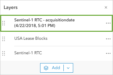
Tip: If you inadvertently added an additional or wrong layer, you can remove it: point to that layer, click Options, and choose Remove. You can then use Image collection explorer again to add the correct layer.
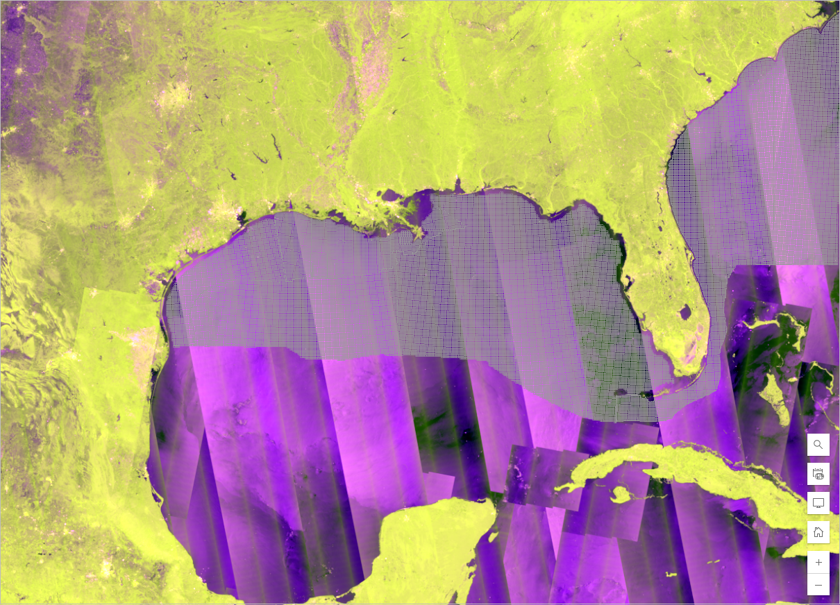
- In the Layers pane, point to the Sentinel-1 RTC layer and click Hide Sentinel-1 RTC to turn it off.
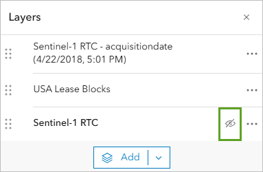
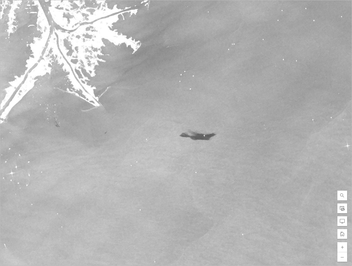
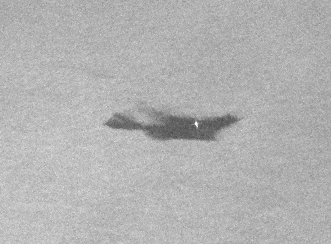
The map now displays Sentinel-1 RTC – acquisitiondate (4/22/2018, 5:01 PM). This layer contains the single SAR image you selected.
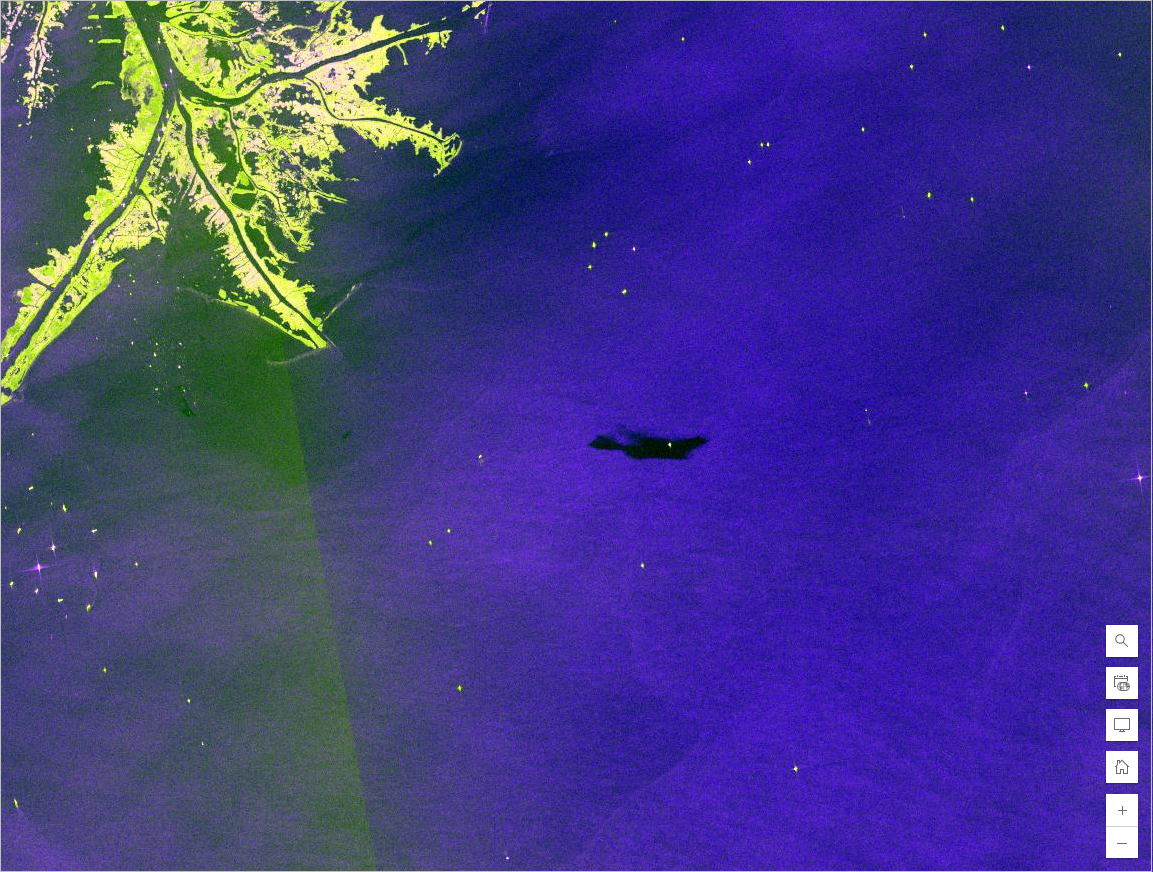
In black, you can see the elongated Taylor Energy oil slick starting from within the MC20 lease block and extending in the east direction.
Apply on-the-fly preprocessing
A SAR image can be displayed differently based on the options you select and the preprocessing you perform on it. You’ll prepare your imagery optimally for oil slick detection.
Sentinel-1 RTC data provides dual polarization VV-VH products. You’ll choose VV polarization, which is preferred for oil slick detection, as it provides strong radar backscatter contrast between the oil slick and surrounding water (see Alpers and Espedal).
There are a variety of techniques to improve the quality of SAR images. You’ll apply a preprocessing step that eliminates speckle noise (a grainy salt-and-pepper pattern common in SAR imagery), converts the data to decibel (dB) scale, and normalizes it to a range between 0 and 255. This preprocessing will be performed on-the-fly for efficiency.
- In the Layers pane, confirm that the Sentinel-1 RTC – acquisitiondate (4/22/2018, 5:01 PM) layer is selected. Click the Processing templates button on the right ribbon.
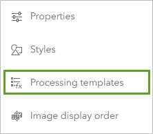
The Processing templates pane lists several options to change the appearance of an image layer.
- In the Processing templates pane, choose VV dB with Despeckle Normalized.
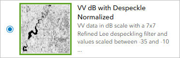
The Processing templates option offers a range of pre-defined on-the-fly functions for imagery visualization and unit conversions. The SAR-specific VV dB with Despeckle Normalized rendering displays the VV polarization and applies the preprocessing steps listed earlier.
- In the Processing templates pane, click Done.
The VV dB with Despeckle Normalized rendering applies.
Next, you’ll rename the image layer to give it a more descriptive name.
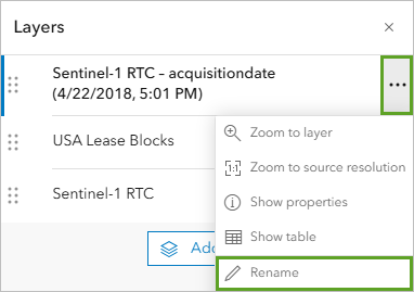
- Point to the Sentinel-1 RTC – acquisitiondate (4/22/2018, 5:01 PM) layer, click Options, and choose Rename.
- In the Rename window, replace the existing text with Sentinel-1 RTC Preprocessed (4/23/2018).
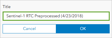
- Click OK.
- On the left ribbon, click Save and open and choose Save.
You added an image layer to your map showing the Taylor Energy oil slick in April 2018 and you optimally preprocessed the layer for oil slick detection.
Apply a pretrained deep learning model
You are now ready to perform the deep learning analysis to extract the oil slick. You’ll use a pretrained deep learning model from ArcGIS Living Atlas and apply the model through the ArcGIS Image for ArcGIS Online capability. With ArcGIS Image for ArcGIS Online, you can publish raster or imagery data to your ArcGIS Online organization and perform various analyses on it.
When running a deep learning model, you can shorten the processing time by applying it to a smaller extent. In this blog tutorial, you’ll do that by zooming in closer to the oil slick.
- Click the Zoom In button twice and pan to view the oil slick at a smaller extent.
The deep learning model will run on the current extent. First, you’ll save the map to your Oil Slick Detection folder.
- On the left ribbon, click Save and open and choose Save.
Run a deep learning tool
Next, you’ll set up the Classify Pixels Using Deep Learning tool, run it, and style its output.
- In the Layers pane, confirm that the Sentinel-1 RTC Preprocessed (4/23/2018) layer is selected. On the right ribbon, click Analysis button.
The Analysis pane appears.
- In the Analysis pane, click Tools.
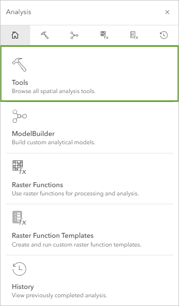
Tip: To access the Raster Analysis tools, you need to have the ArcGIS Image for ArcGIS Online capability enabled. If you don’t see the Raster Analysis option, confirm with your ArcGIS Online organization administrator whether you have sufficient permissions.
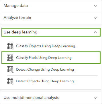
- In the Tools pane, expand Use deep learning and click Classify Pixels Using Deep Learning.
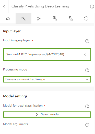
In the Classify Pixels Using Deep Learning tool pane, set the following parameters:
- For Input imagery layer, ensure that Sentinel-1 RTC Preprocessed (4/23/2018) is selected.
- For Processing mode, confirm that Process as mosaicked image is selected.
- For Model for pixel classification, click Select model.
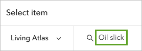
- In the Select item window, next to My content, click the drop-down arrow and choose Living Atlas.

A list of deep learning packages with pretrained deep learning models appears.
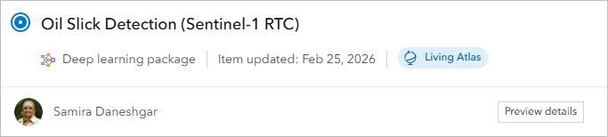
- In the search field, type “Oil slick”.
- In the list of results, identify the Oil Slick Detection (Sentinel-1 RTC) deep learning package. Select it then click Confirm.
In the Classify Pixels Using Deep Learning tool pane, the Model for pixel classification parameter updates to the package you selected.
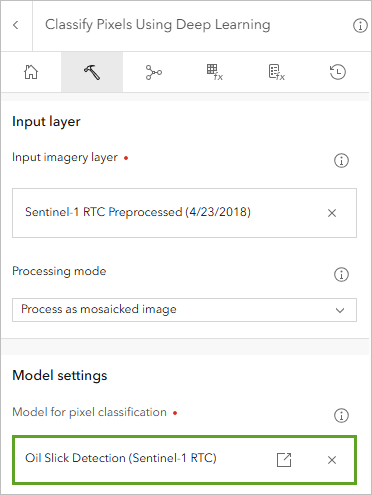
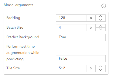
The model arguments are also populated automatically based on the model chosen.
- For Model arguments, keep the default settings.
- Set the following parameters:
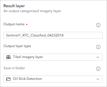
- For Output name, type “Sentinel1_RTC_Classified_04232018” followed by your name or initials (for example, “Sentinel1_RTC_Classified_04232018_YN”).
- For Output layer type, confirm that Tiled imagery layer is selected.
- For Save in folder, choose your Oil Slick Detection folder.
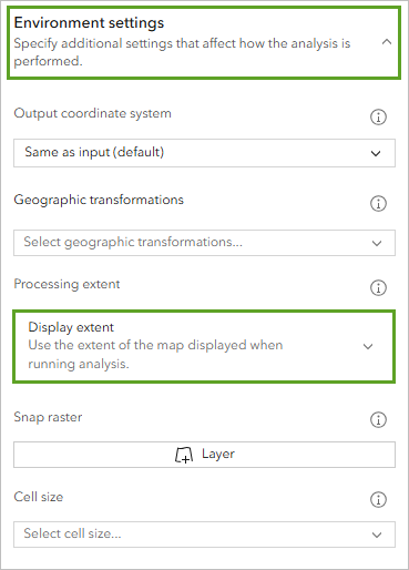
- Expand the Environment settings tool pane, and select Display extent for Processing extent.
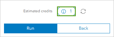
- Click Estimate credits to see the number of credits that will be consumed when running the model.

Estimated credits shows that the tool will consume 1 credit.
Note: Any time you perform analysis in ArcGIS Online, there is a cost in credits for the compute resources. The cost of running a tool in ArcGIS Image for ArcGIS Online depends on the complexity of the analysis and the number of pixels to be processed. One way to control cost is by reducing the area to be processed by zooming in and selecting Display extent for Processing extent before running the analysis.
- Click the Run button. The tool may take a few minutes to run.
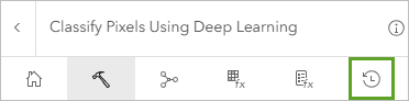
Tip: To check the job progress, click History in the Classify Pixels Using Deep Learning pane.
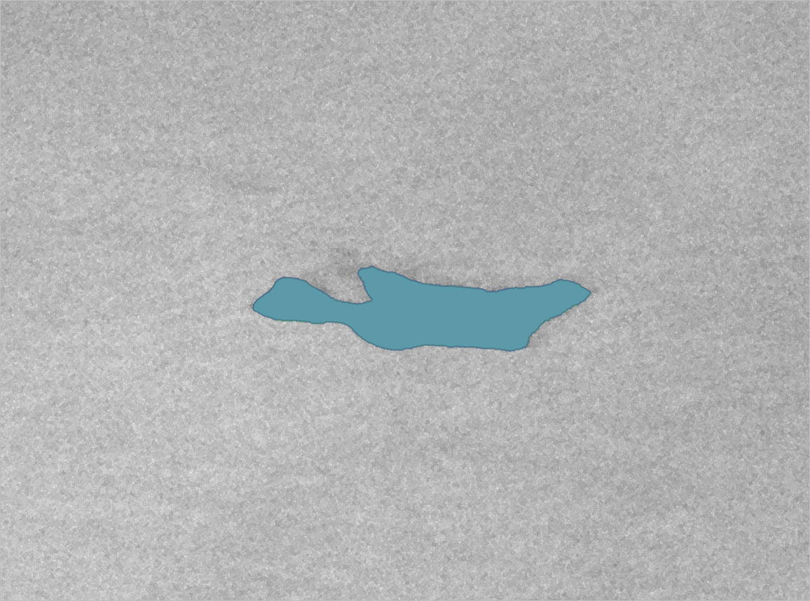
When the process is complete, the result layer is listed in the Layers pane.
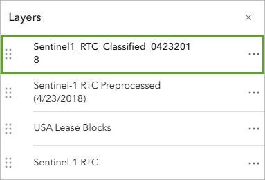
You can now see the extracted oil slick pixels in green displaying on top of your SAR imagery layer.

- On the left ribbon, click Save and open and choose Save.
Convert the extracted oil slick pixels to a vector layer
Now that you’ve extracted the oil slick pixels, it is recommended to vectorize them, or convert them to polygons stored in a hosted feature layer. A feature layer will be easier to reuse in further analyses in ArcGIS Online or ArcGIS Pro, such as computing an accurate area estimation. You’ll also be able to share it with your colleagues or community.
- In the Classify Pixels Using Deep Learning pane, click the back button to return to the Tools pane.
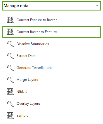
- In the Tools pane, expand Manage data and click Convert Raster to Feature.
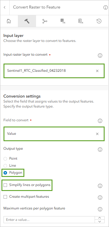
- In the Convert Raster to Feature pane, set the following parameters:
- For Input raster layer to convert, confirm that Sentinel1_RTC_Classified_04232018 is selected.
- For Field to convert, confirm that Value is selected.
- For Choose output type, click Polygon.
- Uncheck Simplify lines or polygons.
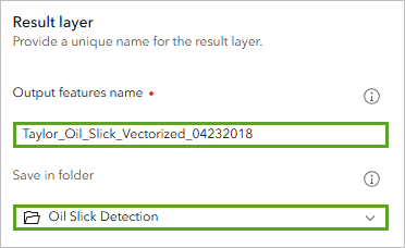
- Under Result layer, set the following parameters:
- For Output features name, type “Taylor_Oil_Slick_Vectorized_04232018” followed by your name or initials (for example, “Taylor_Oil_Slick_Vectorized_04232018_YN”).
- For Save in folder, confirm that your Oil Slick Detection folder is selected.
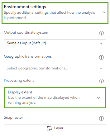
- Expand the Environment settings, and for Processing extent, confirm that Display extent is selected.
- Click Estimate credits.

The tool will consume 1 credit.
- Click Run. The Convert Raster to Feature tool runs for a few moments.
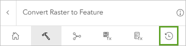
Tip: To check the job progress, click History in the Convert Raster to Feature pane.
When the process is complete, the result layer is listed in the Layers pane.
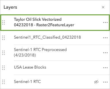
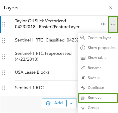
- In the Layers pane, point to the Taylor Oil Slick Vectorized 04232018 – Raster2FeatureLayer layer, click Options, and choose Remove.
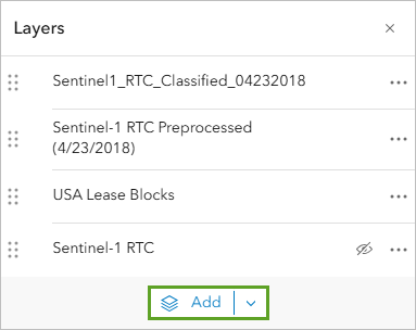
- In the Layers pane, click the Add button.
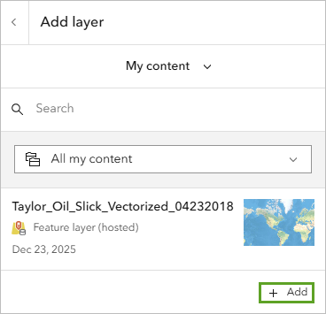
- Add Taylor_Oil_Slick_Vectorized_04232018 from My content.
- Click the back button to return to the Layers pane.

Finalize the vectorized oil slick layer
Next, you’ll finalize the Taylor_Oil_Slick_Vectorized_04232018 layer. The layer contains two polygons, representing either the oil slick or the non-oil slick areas in the extent.
- On the map, click a few points to visualize the polygons and their associated information.
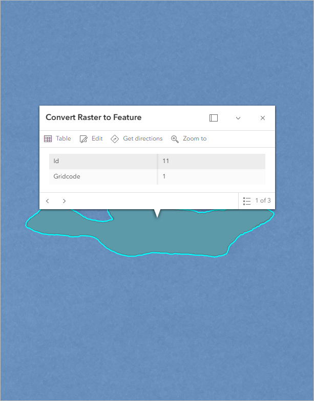
The oil slick polygon have a Gridcode attribute value of 1. The non-oil slick polygon has a Gridcode attribute value of 0. You’ll filter the layer to keep only the polygons with a Gridcode value of 1.
- In the Layers pane, confirm that the Taylor_Oil_Slick_Vectorized_04232018 layer is selected. Click the Filter button on the right ribbon.
- In the Filter pane, create the expression gridcode is 1 and click Save.
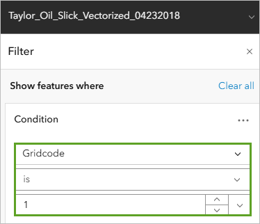
The layer now displays only the polygon that corresponds to the oil slick.
Tip: Sentinel-1 SAR detection of floating oil is challenged by the possibility of false positives, which can result in dark areas like oil. Low-wind areas, biogenic oil films, rain cells, grease ice or frazil sea ice, surface current shears, wind sheltering by land, upwelling zones, and internal waves can all appear dark in Sentinel-1 imagery and be mistaken for oil. If false positives occur, you can use the Edit button on the right ribbon to select and delete false positive polygons from the results.
Next, you’ll change the style of the layer to make it more visible.
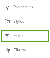
- In the Layers pane, confirm that the Taylor_Oil_Slick_Vectorized_04232018 layer is selected. Click the Styles button on the right ribbon.
- In the Styles pane, under Pick a style, for Location (single symbol), click Style options.
- Under Location (Single symbol), click Symbol style.
- In the symbol style window, for the Fill color tab, click No Color.
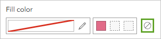
- For the Outline color tab, click Select color.

- Choose the red color (#FF0000).
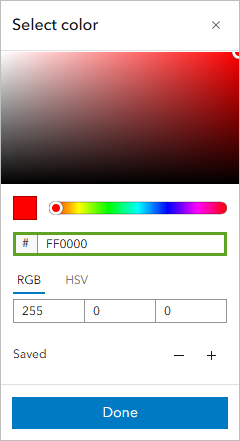
- Click Done. In the Styles pane, click Done and click Done.
- In the Layers pane, turn off the Sentinel1_RTC_Classified_04232018 layer.
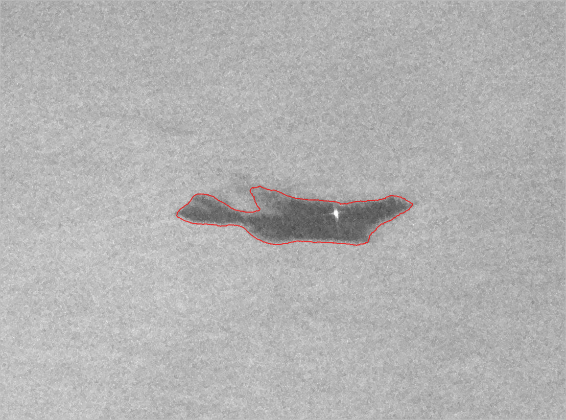
You can now see the oil slick polygon outlined in red and displayed over the SAR image.
You’ll save the polygon layer so that the enhancements you’ve made to it are recorded in your ArcGIS Online content.
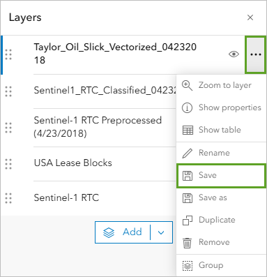
- In the Layers pane, point to the Taylor_Oil_Slick_Vectorized_04232018 layer, click Options, and choose Save.
You’ll remove the rest of the layers from the map, as you don’t need them any longer.
- In the Layers pane, point to the Sentinel1_RTC_Classified_04232018 layer, click Options, and choose Remove.
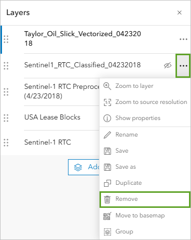
- Similarly, remove the Sentinel-1 RTC Preprocessed (4/23/2018), USA Lease Blocks, and Sentinel-1 RTC layers.
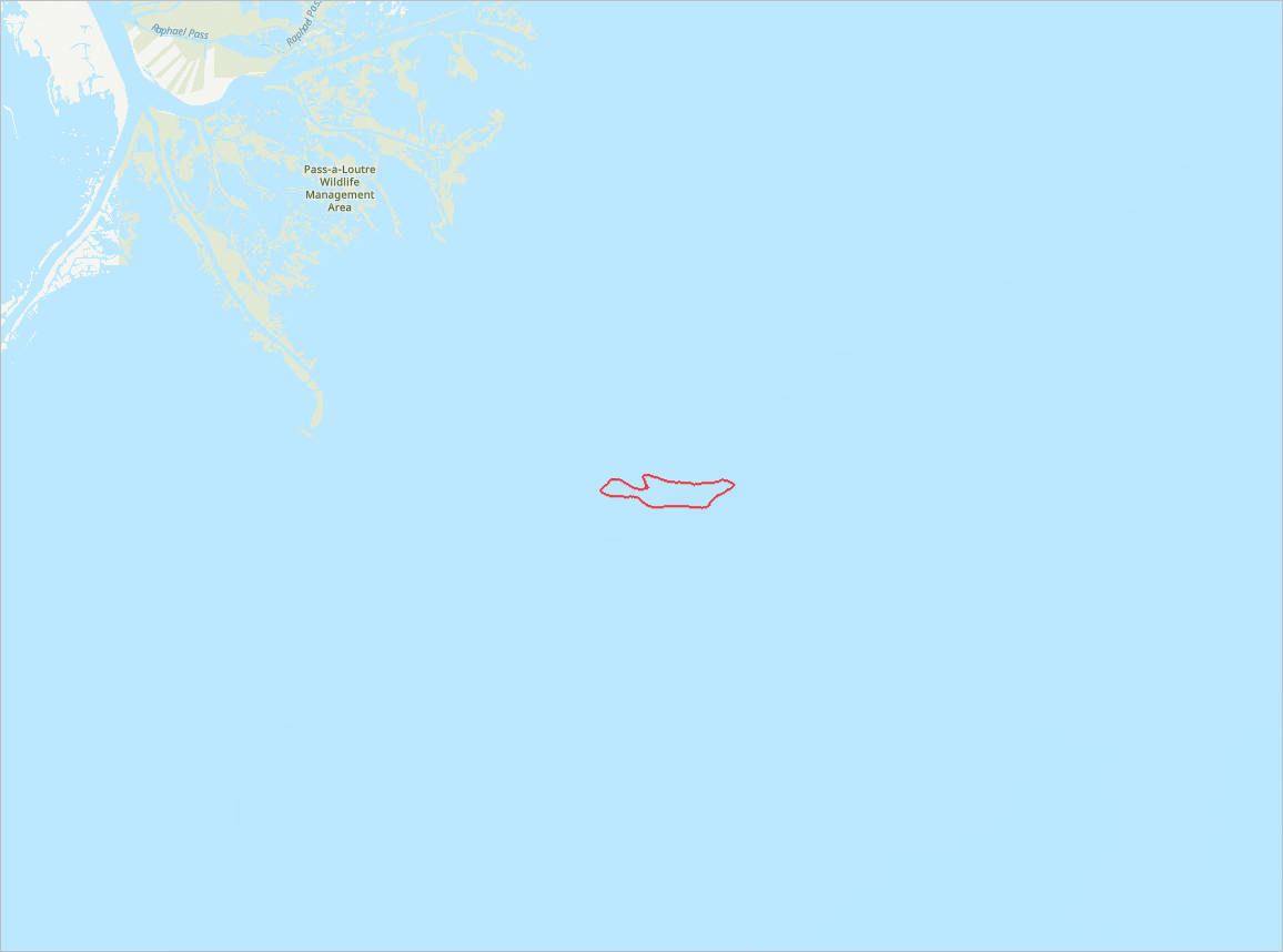
- Zoom out two or three times until you see some of the land for reference.
You can now see the oil slick polygon displayed over the topographic basemap.
- On the ribbon, click Save and open and choose Save.
The web map is now ready to share with your colleagues or community.
Tip: To make the web map publicly available, on the left ribbon, click the Share map button, and adjust the sharing settings.

Finally, you’ll organize the data in your Oil Slick Detection folder.
- In the top bar, click menu button and choose Content.
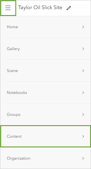
- If necessary, open your Oil Slick Detection folder.
You’ll delete the hosted imagery layer that you generated as part of this workflow, since you don’t need it any longer.
Caution: It is important to delete hosted imagery items you don’t need to avoid consuming credits for their ongoing storage.
- Check the box next to Sentinel1_RTC_Classified_04232018 to select the layer.
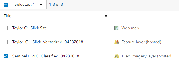
- Click Delete.

At this point, your folder contains:
- The vectorized oil slick layer (Taylor_Oil_Slick_Vectorized_04232018).
- The map that contains the vectorized oil slick layer (Taylor Oil Slick Site).
You’ve successfully extracted an oil slick from an imagery layer using a pretrained deep learning model. You also converted it to a vector layer. You can now use the resulting layer for further analysis. You also created a web map showcasing the layer that you can share with your colleagues or community.
In this blog tutorial, you extracted an oil slick using a Sentinel-1 RTC dynamic imagery layer and a pretrained deep learning model. You first created a web map containing the Sentinel-1 RTC layer. You then selected your imagery of interest and preprocessed it on the fly. Finally, you applied a pretrained deep learning model to it to extract the oil slick and converted the result to a vector layer.
Moving forward, you could use the same workflow repeatedly to analyze data over time and gain further insights into the extent of the oil slicks caused by the Taylor Energy oil spill over the past 15 years. For example, a dashboard of the 2018 oil slicks has been created, showing their estimated area and volume. This workflow would also apply to any other oil slick, and could help initiate and monitor the oil-spill cleaning process to protect the marine environment.
Moving forward, you could use the same workflow repeatedly to analyze data over time and gain further insights into the extent of the oil slicks caused by the Taylor Energy oil spill over the past 15 years. For example, a dashboard of the 2018 oil slicks has been created, highlighting their estimated area and volume. The dashboard clearly demonstrates the variability in oil slick spatial extent, surface coverage, and estimated volume over time.
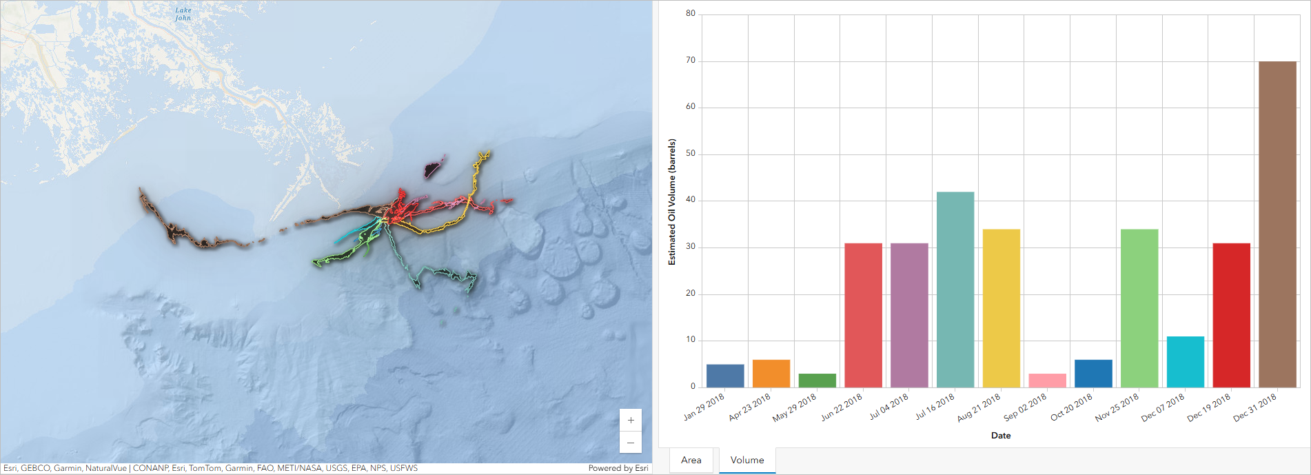
Taylor Energy Oil Spill: 2018 Monthly Oil Slick Extent and Volume Dashboard
Area tab: Displays the total detected oil area in square kilometers by date.
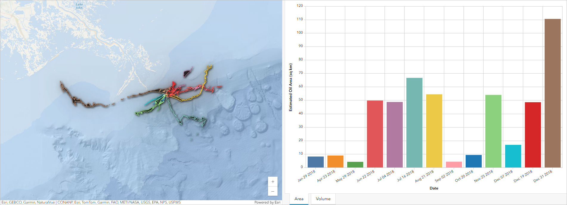
Volume tab: Presents estimated oil volumes in barrels, derived from the detected surface area using a uniform thickness assumption of 0.1 µm—a conservative, lower-bound estimate representing the thickness of oil forming a visible sheen on water. These estimates are intended for relative comparison rather than precise quantification.
This workflow is applicable to any oil slick and can support efforts to monitor and manage oil spill response, helping to protect the marine environment.
Additional resources
You can find more tutorials in the tutorial gallery.
Explore additional raster analysis blog tutorials using Living Atlas imagery content.
Learn more about SAR in Guide: Fundamentals of Synthetic Aperture Radar.
Acknowledgements
- Sentinel-1 RTC layer: Copernicus Sentinel-1 data from European Space Agency, sourced from the Microsoft Planetary Computer and accessed via ArcGIS Living Atlas of the World.
- USA Lease Blocks layer: Outer Continental Shelf (OCS) lease block data from US Department of Energy’s Bureau of Ocean and Energy Management (BOEM) accessed via ArcGIS Living Atlas of the World.
- Alpers and Espedal, H. (2004). Oils and Surfactants. Synthetic Aperture Radar Marine User’s Manual. 263-277.
- Topographic sources: Esri, HERE, Garmin, FAO, NOAA, USGS, Intermap, METI, © OpenStreetMap contributors, and the GIS User Community

Article Discussion: