Enabling communities around the world with on-demand urban heat mapping.

Heat waves and urban heat island effects are increasing heat-related illnesses and deaths worldwide. According to the World Health Organization, heat-related deaths among people over age 65 increased by 85% between 2000 and 2021. While individuals can take steps to protect themselves from extreme heat, city planners and landscape architects can reduce heat risk across entire communities by decreasing paved surfaces, increasing water features, and planting more trees and vegetation. These strategies can be highly effective but are often expensive, making it important to understand where heat risk is greatest so resources can be targeted effectively.

In Part 1 of this blog series, you learned how to utilize Landsat Level-2 multispectral imagery to map urban heat islands, but that only tells part of the story. In this blog, you will utilize ArcGIS Living Atlas of the World data, as well as the tools available in ArcGIS Online Map Viewer, to map out an urban heat risk index of Monterrey, Mexico. With this data, you’ll be able to garner a broader understanding of where the urban area is most vulnerable to heat risk.

Quick links

Use the links below to navigate to different sections of this article.

• Terms of Use
• System Requirements
• Calculate Surface Heat Zones
• Calculate Vegetated Area Zones
• Calculate Population Data
• Create a Heat Risk Index
• Assess Results

Terms of Use

The Mexico AGEB Boundary layer used in this workflow is intended to support online visualization and analysis only. Users are not permitted to export data for offline use.

System Requirements

• An ArcGIS Online organizational account with credits*
• A minimum of a Professional User Type with a Publisher role.
• Analysis-optimized imagery layers enabled for your organization**
• Completion of Part 1 of this workflow with all the intermediate products saved in your content.

*This tutorial consumes a total of approximately 19 credits. The number of credits is determined by the geographic extent and how many index variables are included.

**Analysis-optimized imagery layers provide scalability for larger and more diverse workflows. This capability must be enabled to avoid size constraints and allow the heat risk index creation to scale appropriately. See ArcGIS Living Atlas ready-to-use imagery layers for analysis for more information, including how to enable imagery layers optimized for analysis.

Calculate Surface Heat Zones

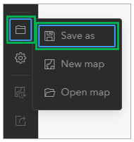
Step 1 – Start by creating a new web map in ArcGIS Online to include all your layers and conduct your analysis. Sign into ArcGIS Online and click on Map found on the ribbon. Once your new untitled map is open, find the Save and Open option on the left-side ribbon. Click it, then click Save as.

Title your map “Monterrey Heat Risk Index” and give it the tags, “Monterrey“, “Heat Island“, and “Heat Risk Index“. Optionally, give it a descriptive summary such as, “A map of data used to compile a heat risk index for Monterrey, Mexico”. Click Save.

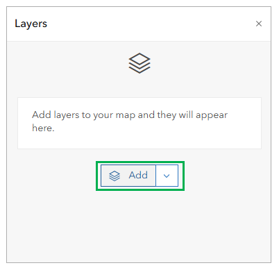
Step 2 – Add the final surface heat raster created in Part 1. Click Add in the Layers pane.

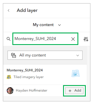
Search My Content for “Monterrey_SUHI_2024” and click Add on the item.

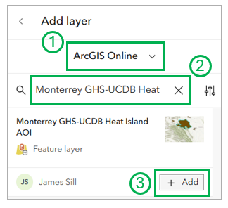
Step 3 – With the urban heat map added to your map, you’ll also need to add the area of interest (AOI) from Part 1. Navigate back to the Layers pane and click Add again.

1. This time, use the drop down to search ArcGIS Online.
2. Type in “Monterrey GHS-UCDB Heat Island AOI“.
3. Find the matching item and click Add.

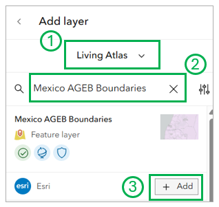
Step 4 – You will now add your zone data from the Living Atlas of the World. Navigate to the Layers pane and click Add again.

1. This time, use the drop down to search Living Atlas.
2. Type in “Mexico AGEB Boundaries“.
3. Find the matching item and click Add.

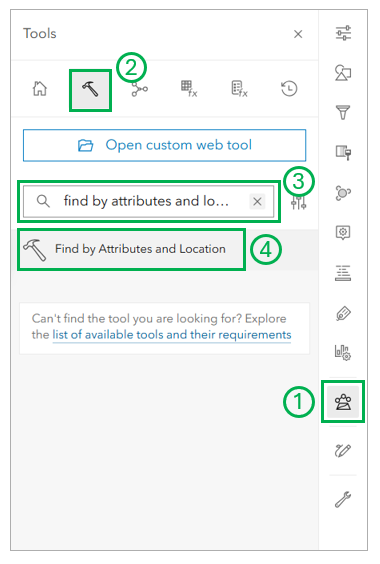
Step 5 – Now that you have your AOI and your zone data in the map, you can select the zones that will be used in the analysis.

1. Navigate to the ribbon the right-hand side and click on Analysis.
2. Click on Tools in the top ribbon.
3. Search for “find by attributes and location“.
4. Click the tool with the matching name.

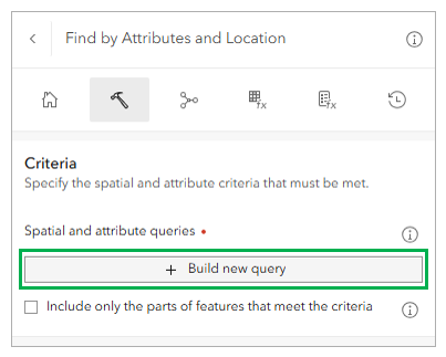
With the Find by Attributes and Location tool open, click on Build new query under the Criteria section.

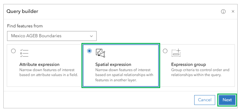
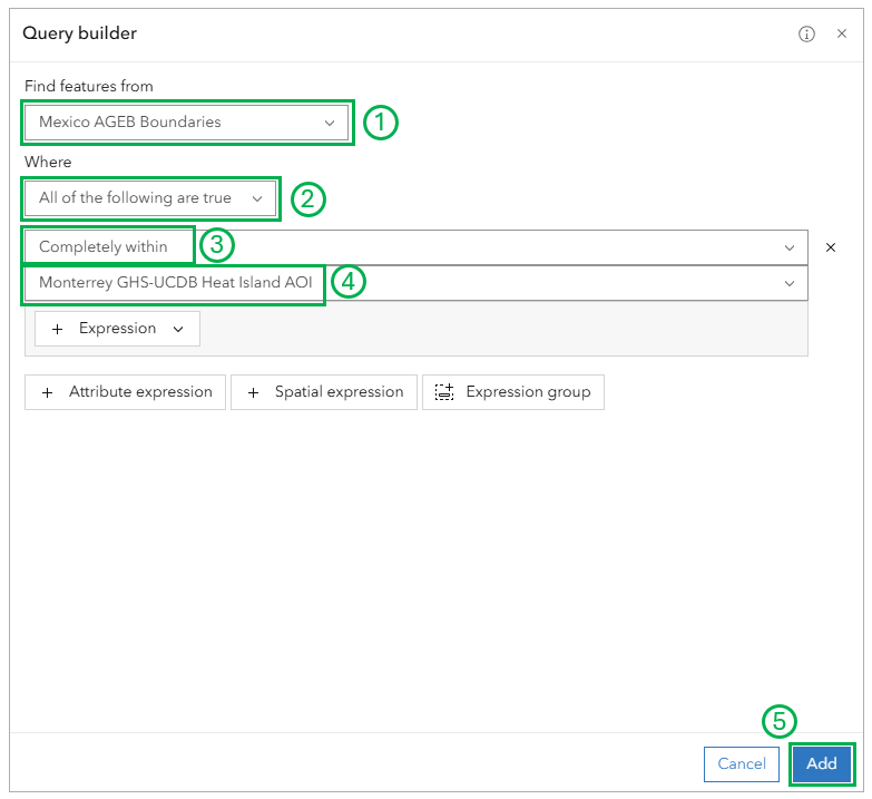
This will open a new Query builder window. Select the Spatial expression option and click Next.

Your query should have the following options:

1. For Find features from, make sure the Mexico AGEB Boundaries layer is selected.
2. For the Where option, make sure the drop down reads All of the following are true.
3. Open the relationship box to select the Completely within option.
4. Finally, make sure the relationship is pointing to the Monterrey GHS-UCDB Heat Island AOI layer
5. Click Add.

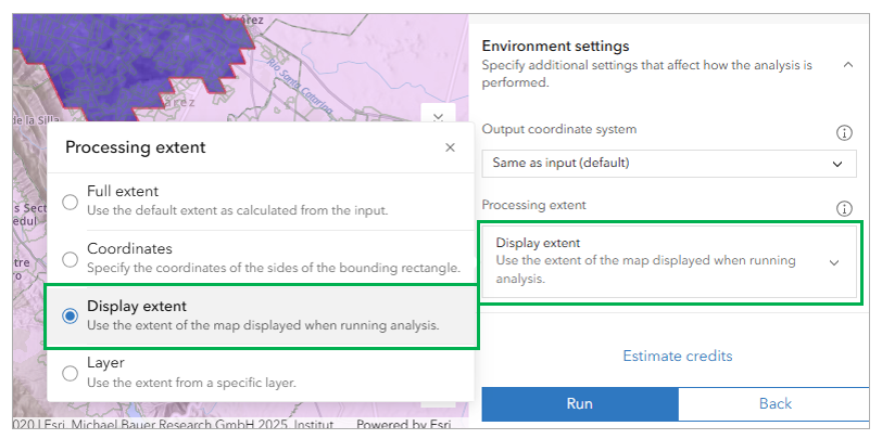
Give it the output name “Monterrey_AGEB_Zones“. Open the Environment settings dropdown and navigate to the Processing extent option. Set it to Display extent (note: when running with this option, ensure that the entire AOI is within your display before clicking Run).

Navigate to the bottom of the tool and click Estimate credits. It should estimate the cost at around 2.1 to 2.2 credits. Once the credit value is returned, click Run.

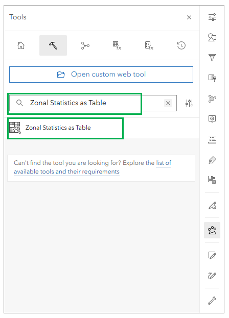
Step 6 – With the zone data in the map, you are ready to begin running your analysis. Navigate back to the Tools tab in the Analysis pane and search for “Zonal Statistics as Table” and open the tool with the matching name.

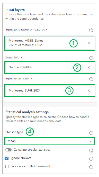
1. For the Input zone rasters or features parameter, select the Monterrey_AGEB_Zones layer you created in the previous step.
2. In the Zone Field parameter, select the Unique Identifier field from the zone data.
3. Select the Monterrey_SUHI_2024 raster that came from Part 1 for the Input value raster parameter.
4. Set the Statistic type to Mean.

Leave everything else the same and give your output table the name “Monterrey_AGEB_SUHI“. Click Estimate credits. It should estimate the cost at around 1 credit. Once the credit estimation finishes, click Run.

Calculate Vegetated Area Zones

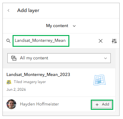
Step 1 – To calculate the vegetated areas to use as an input for your index, you’ll run a normalized difference vegetation index (NDVI) on Landsat satellite imagery to create a vegetation mask. Start by navigating to the Layers pane and clicking Add. You should have an aggregate mean of Landsat data over Monterrey from Part 1. Search for “Landsat_Monterrey_Mean” in your content and click Add on the item.

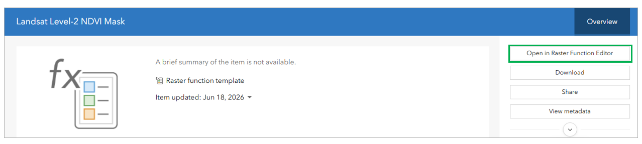
Step 2 –  With the aggregate Landsat data in your map, you can now run the NDVI mask function on it. Click this link to open the item page for the Landsat Level-2 NDVI Mask raster function template. With the item page open, click Open in Raster Function Editor.

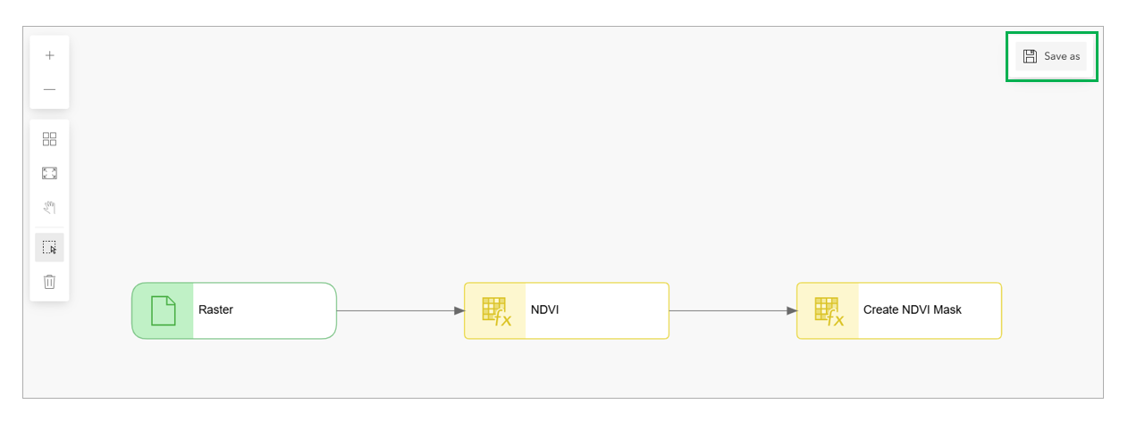
In the Raster Function Editor window, you can look at the different raster functions and their parameters used in the NDVI mask function. Once you’re done examining the functions, click Save as then Save to save a copy in your content.

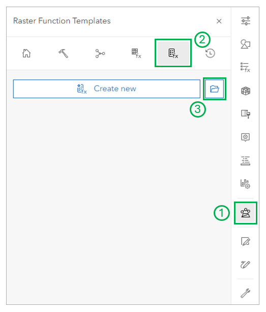
Step 3 – Return to your Monterrey Heat Risk Index map.

1. Navigate to the Analysis tab.
2. Click on Raster Function Templates on the top ribbon.
3. Click on Browse Raster Function Templates.

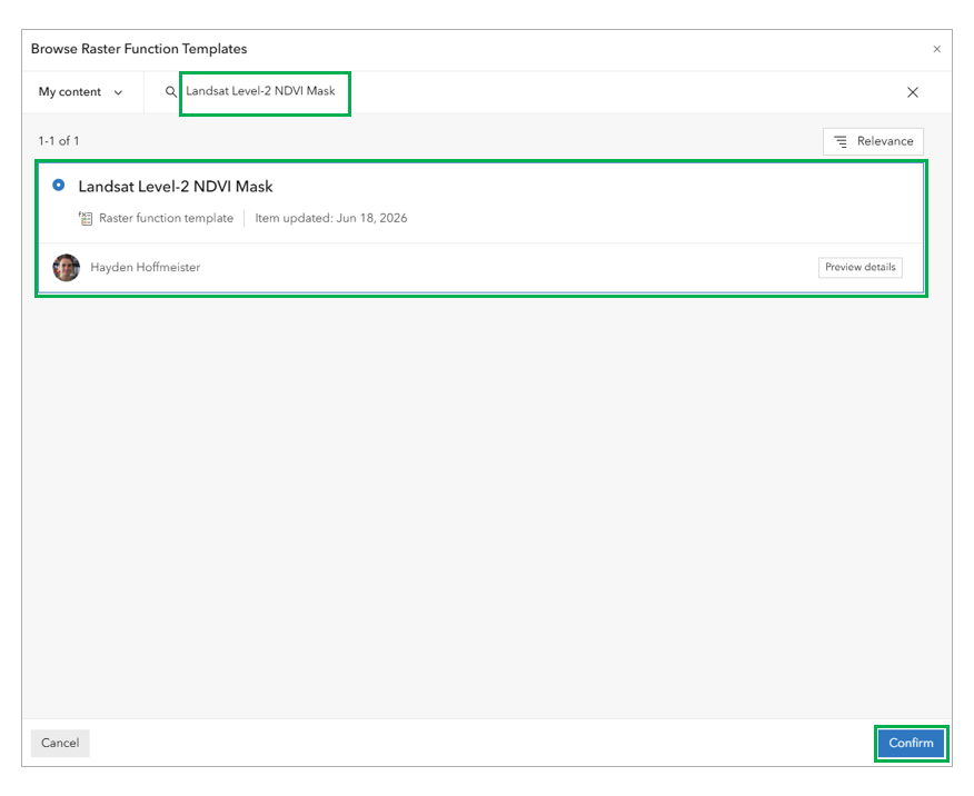
Search your content for “landsat level-2 NDVI mask” and click on the result to select it. Then, click Confirm.

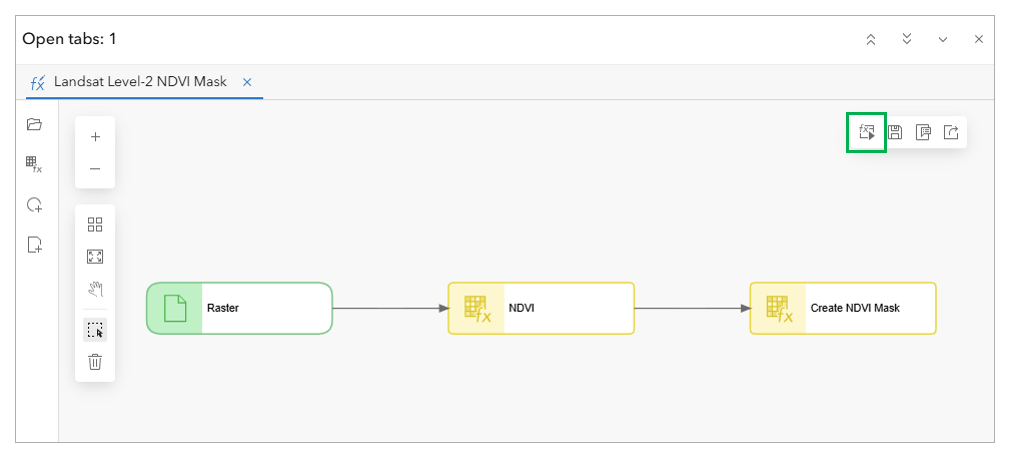
The raster function template will automatically open in a new window. Find the small dialogue box in the upper right-hand corner and click the Open to Run option. This will open the raster function template in the Tools tab.

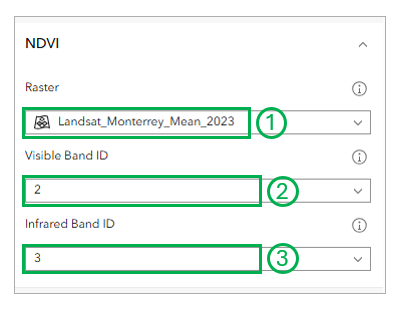
1. For the Raster parameter, select the Landsat_Monterrey_Mean aggregate raster.
2. You’ll also need to set the band IDs: for the Visible Band ID use the drop down to select 2.
3. For the Infrared Band ID use the drop down to select 3.

Give your output the name “Monterrey_Vegetated_Area”. Click Estimate credits; the estimated cost should be around 1 credit. After the estimation completes, click Run.

Note: the band IDs are dependent on the raster dataset you’re using. If you wanted to run this raster function template against a single Landsat Level-2 scene, the visible and infrared band IDs would be 4 and 5 respectively.

Step 4 – Once you have the non-built areas raster in your map, you’ll need to run the same zonal statistics operation on it as you did on the surface heat raster. Navigate back to the Tools tab in the Analysis pane and open the Zonal Statistics as Table tool again.

1. Set the Input zone raster or features to the Monterrey_AGEB_Zones again.
2. Set the Zone field to the Unique Identifier field.
3. Set the Input value raster as the Monterrey_Vegetated_Area raster.
4. Set the Statistics type to Mean again.

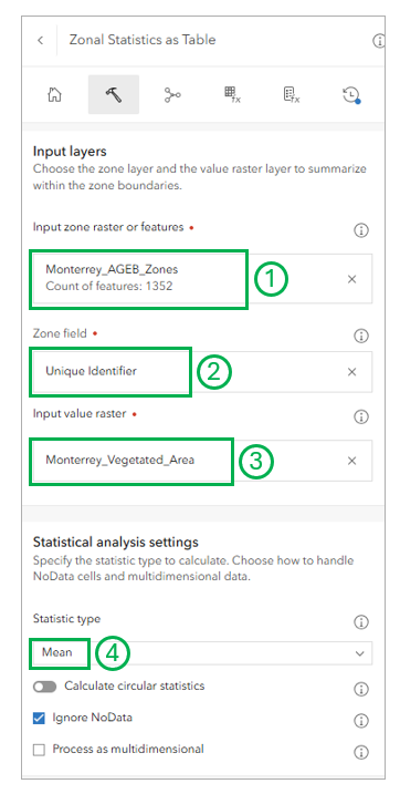
Name the output “Monterrey_AGEB_Vegetated” and click Estimate credits. The estimated cost should be around 1 credit. Once the estimation finishes, click Run.

Calculate Population Statistics

The data being utilized in this version of the workflow draws population statistics from both the INEGI’s Marco Geoestadístico data, as well as the global WorldPop population data. For the purposes of this specific workflow and area of interest, these are the best available datasets for you to leverage. Using the methods outlined in this section, the workflow can easily be enhanced by other population statistics if there is better data available to you for this area of interest, or another area of interest you may want to calculate a heat risk index for.

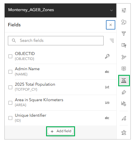
Step 1 – The Mexico AGEB Boundaries data contains population data for each zone by default. You can use this data to calculate population density, but first you need to add a population density field. Select your Monterrey_AGEB_Zones layer in the Layers pane. Then, on the right-hand ribbon, click Fields. In the Fields pane, click Add field.

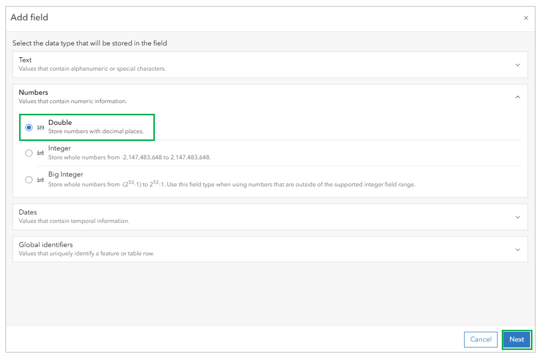
An Add field window should open. Under the Numbers drop down, click the Double option, and then click Next.

1. For the Field name, write in “pop_den“.
2. For the Display name, write in “Population Density“.
3. Set the Default value to “0” (optional).
4. You can add a short description to the field that reads “Population per square kilometer calculated using the population field and the area field” (optional).
5. You can also change the “Field value type” to “Count or Amount” (optional).

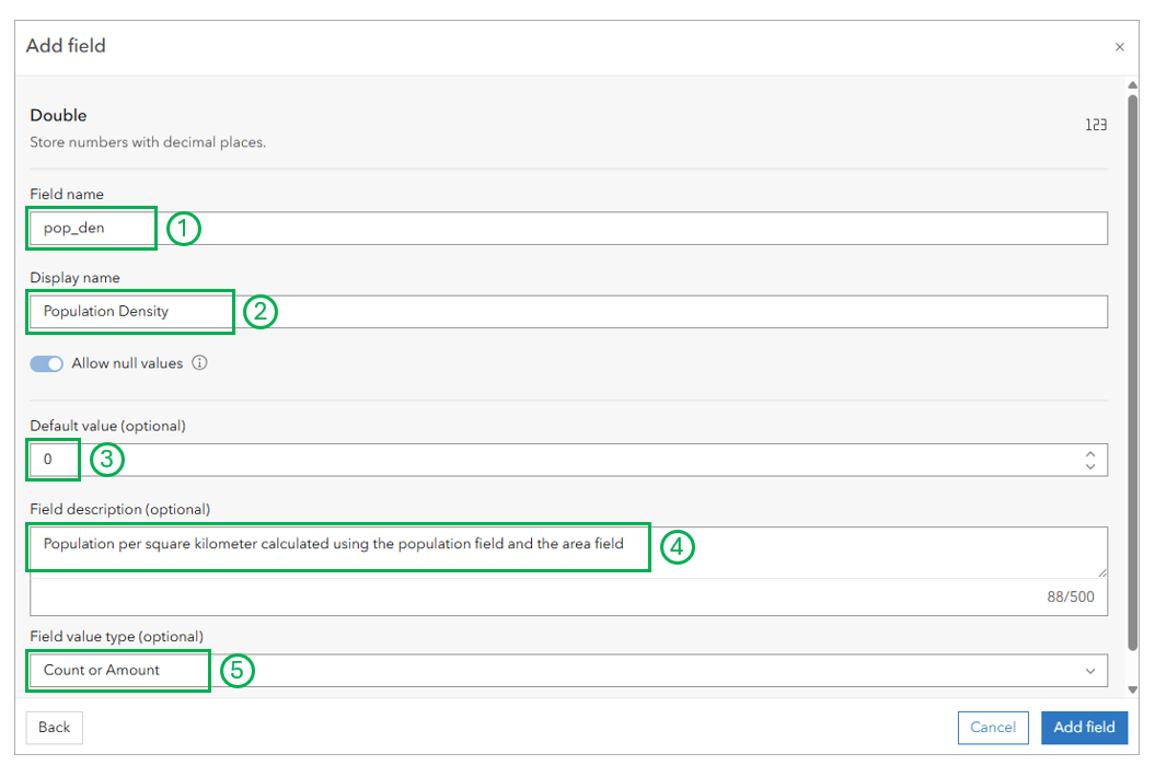
Once all the parameters are filled in, click Add field.

Step 2 – Now that the zone data has a population density field, you can calculate the population density to fill in that field. Navigate to the Layers pane, and find your Monterrey_AGEB_Zones layer. Click on the ellipses and then Show table in the drop-down menu. This will open the table for your zone data.

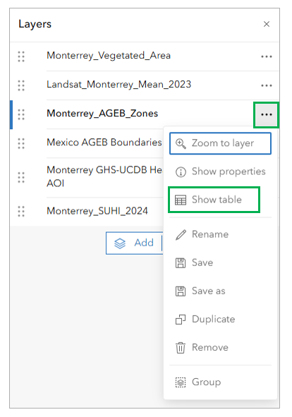
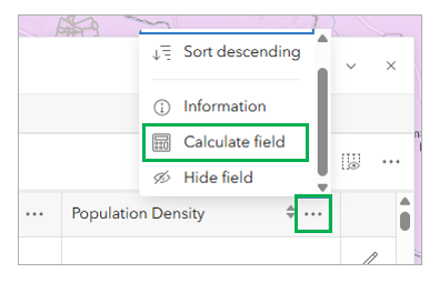
In the table, find the Population Density field you created (it should be empty at this point). Next to the field name in the top row, click on the ellipses and then click Calculate Field.

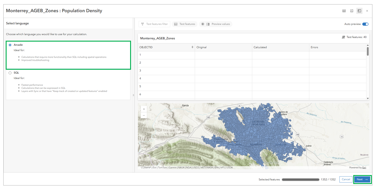
The field calculator window should now be opened. There are a few different ways to calculate the population density; for this workflow you’ll use Arcade. Click on the  Arcade option then click Next. You won’t apply any filter, so click Next again. 

In the Arcade Expression dialogue box, use the following expression to calculate the field:

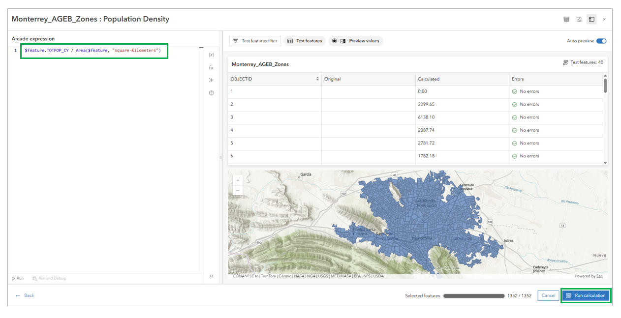
This expression divides the population of each zone by that zone’s geometric area in square kilometers. The field calculator will automatically show you a preview of your calculation operation. Use this to ensure there are no issues or errors. Once you’re confident in the calculation, click Run calculation.

Step 3 – With the population density calculated, you can now add more population data from the Living Atlas of the World to include in your index. Navigate to the Layers pane and click Add again. Use the drop down to select the Living Atlas option and search for “Global Estimated Population Ages 65 and Older in 2020“. Click Add on the item with the matching name.

Step 4 –  You can now  run the same zonal statistics operation on the population raster datasets as you’ve done on your previous raster data. Navigate back to the Tools tab in the Analysis pane and open the “Zonal Statistics as Table” tool again.

1. Set the Input zone raster or features to the Monterrey_AGEB_Zones again.
2. Set the Zone field to the Unique Identifier field.
3. Set the Input value raster as the Global Estimated Population Ages 65 and Older in 2020 raster.
4. Set the Statistics type to Mean.

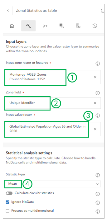
Name the output “Monterrey_AGEB_Over65”, but do not run the tool yet!

Because the spatial reference and cell sizes are different for the population data compared to the data you’ve been using, you’ll want to adjust some of the environment variables.

1. Click on the Environment settings dropdown.
2. For the Output coordinate system parameters, click on the drop down and select the Same as layer option.
3. For the layer, select the Monterrey_SUHI_2024 raster.
4. Then, find the Cell size parameter and select the From layer option.
5. For the layer, select the Monterrey_SUHI_2024 raster again.

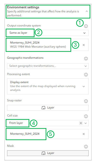
Once your environmental variables are set, click Estimate credits. The cost should be estimated around 1 credit. Once your estimation finishes, click Run.

Combine Into Heat Risk Index

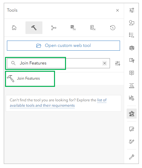
Step 1 – With all the index inputs prepared and in your map, you’re now ready to work on the final heat risk index. You’ll start by joining all the previous datasets together. Navigate to the Tools tab in the Analysis pane and search for “Join Features“. Select the tool with the matching name.

First, you’ll join the heat surface data back to the zones.

1. For the Target layer select Monterrey_AGEB_Zones.
2. For the Join layer select Monterrey_AGEB_SUHI table.
3. In the Join settings dropdown, make sure the Use attribute relationship parameter is checked.
4. For the relationship, set the Target field to Unique Identifier.
5. Set the Join field to ID.
6. Change the Join type to Left join.

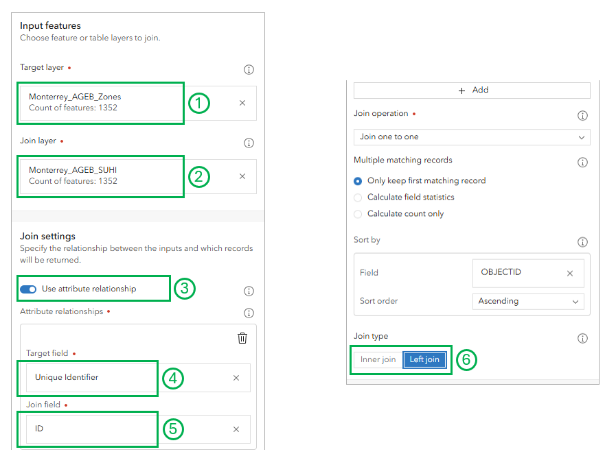
Name the output “Monterrey_AGEB_SUHI_join” and click Estimate credits. The estimated cost should be around 2.7 to 2.8 credits. Once the estimation finishes, click Run.

Step 2 – Next, you’ll join the vegetated area data to the previously joined data. Navigate back to the Join Features tool in the Tools tab in the Analysis pane.

1. Set the Target layer to your Monterrey_AGEB_SUHI_join layer
2. For the Join layer, set it to your Monterrey_AGEB_Vegetated table.

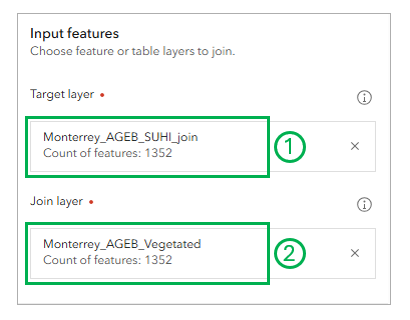
The rest of the join settings and parameters should be the same as the previous operation. Name the output “Monterrey_AGEB_SUHI_Vegetated_join” and click Estimate credits. The estimated cost should be around 2.7 to 2.8 credits. Once the estimation finishes, click Run.

Step 3 – Finally, you’ll join the population Over 65 data to the previously joined data. Navigate back to the Join Features tool in the Tools tab in the Analysis pane.

1. For this operation, set the Target layer to your Monterrey_AGEB_SUHI_Vegetated_join layer.
2. Set the Join layer to your Monterrey_AGEB_Over65 layer.

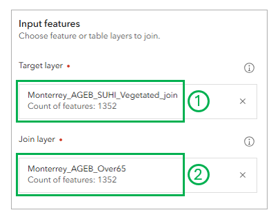
The rest of the join settings and parameters should be the same as the previous operation. Name the output “Monterrey_AGEB_SUHI_Vegetated_Over65_join” and click Estimate credits. The estimated cost should be around 2.7 to 2.8 credits. Once the estimation finishes, click Run.

Step 5 – All the data is now joined together in one layer, but since the tables were created using the same zone features, you’ll have some duplicate fields to clean up.

In the Contents pane, select the Monterrey_AGEB_SUHI_Vegetated_Over65_join layer. Then, on the right-hand ribbon, click Properties, this will open the layer’s properties. In the properties pane, click Information to open the information dropdown menu. Click the icon next to the layer name to go to the item page.

The item page provides useful information and metadata for the item, but also gives users access to more in depth data engineering. You’ll leverage these capabilities to manage the layer’s fields.

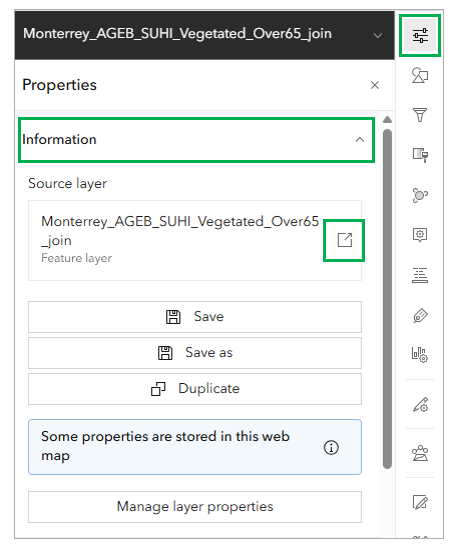
From here, start by clicking on the pencil icon next to the layer name and renaming the layer name to “Monterrey HRI Input“. Then, click on Data in the top ribbon the the right of the name. This will take you to a page that allows you to edit the table and fields of the layer.

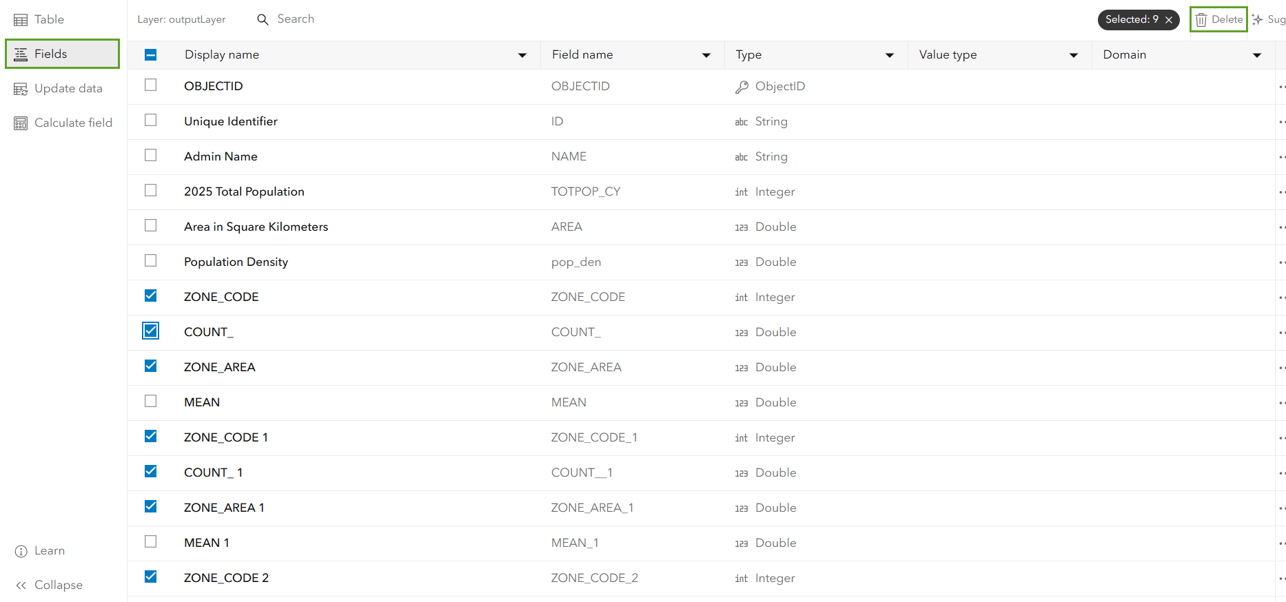
On the lefthand ribbon, click Fields. Examine the fields and notice how there are a variety of duplicate fields. Using the checkbox next to each field, select the following fields:

• ZONE_CODE
• COUNT_
• ZONE_AREA
• ZONE_CODE 1
• COUNT_ 1
• ZONE_AREA 1
• ZONE_CODE 2
• COUNT 2
• AREA  2

Note: DO NOT select any of the MEAN fields. These are not duplicates, they are the unique zonal statistic values calculated for each layer.

Once all the fields are selected, go to the upper righthand corner and click Delete. Confirm you’ve selected the correct fields, then click Delete Fields (9).

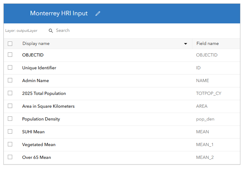
Next, rename each MEAN so it reflects the data it represents. Click on the first mean field named MEAN. This will open the field properties pane. Find the pencil icon next to the name, click it, and rename the field “SUHI Mean” and click Save. Then, rename the remaining mean fields as follows:

• MEAN 1 = NonBuilt Mean
• MEAN 2 = Over 65 Mean

Once you have deleted all the duplicate fields and renamed the mean fields, your fields should look like this:

Close the item tab and return to your map. Locate your old Monterrey_AGEB_SUHI_Vegetated_Over65_join layer in the Layer pane, click on the …, and click Remove.

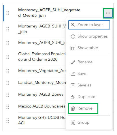
Then click Add in the Layer pane and search your content for “Monterrey HRI Input”. Click + Add on the item to add it back to your map. You have compiled all your data, and you are now ready to create your composite index.

Step 6 – Navigate to the Tools tab in the Analysis pane and search for “Calculate Composite Index” and open the tool with the matching name.

1. For the Input features or table parameter, select your newly added Monterrey HRI Input layer.
2. Under the Input variables parameter, for the first input variable, select the SUHI Mean field and leave everything else default, then click Add.
3. For the next variable, select the Vegetated Mean field and check the Reverse direction box.
4. Add a variable for the Population Density field.
5. Add another variable for the Over 65 Mean field.

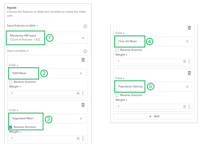
You should have five total input variables. You can leave the “Index settings” at their default values and rename the output to “Monterrey Heat Risk Index”. Click Estimate credits. The cost should be estimated at around 1 to 2 credits. Once the estimation has finished, click Run.

Assess Results

Step 1 – Now that the final heat risk index data is in your map, it’s time to visualize it for analysis. Start by turning off all layers except Monterrey Heat Risk Index. Navigate to the Layers pane on the left hand side, and hove over a layer. Click on the eye icon that appears to hide the layer.

Step 2 – Once all the other layers are turned off, you’ll need to pick the variable you want to visualize. Select the Monterrey Heat Risk Index by clicking on it in the Layers pane. Navigate to the right-hand ribbon and click the Styles button.

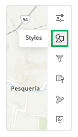
With the Styles pane open, find the Choose attributes section and click on the X next to the Custom attribute.

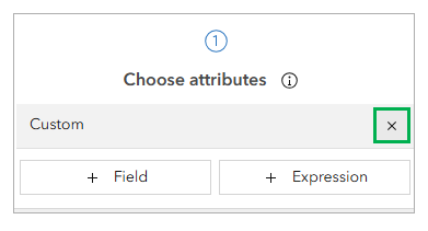
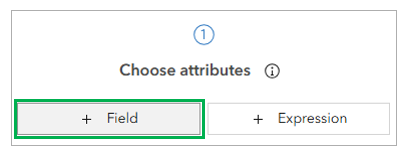
Now, in the same Choose attributes section, click on the + Field button to add a new field to visualize the data.

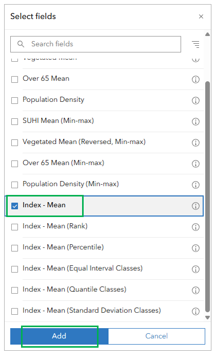
Find the Index – Mean field, select it, then click Add.

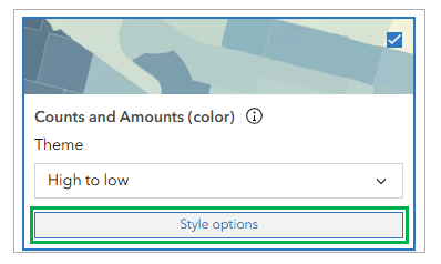
Step 3 – With the proper variable selected to style, it’s now time to visualize it. In the Styles pane, find the Pick a style subsection, and ensure the Counts and Amounts (color) option is selected. Click Style options.

The data should now visualize the index from low to high on a continuous color ramp, but there are a few improvements you can make. First, change the color so it better represents the heat aspect of the data. Find the Symbol style option and click on the pencil icon. With the Symbol style window open, find the Colors option and click on the pencil icon again.

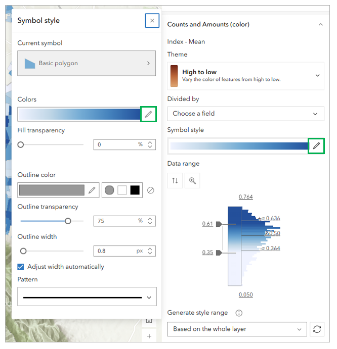
With the Ramp window open, find the Red 2 color ramp along the top row. Click on it, then click Done.

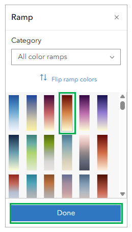
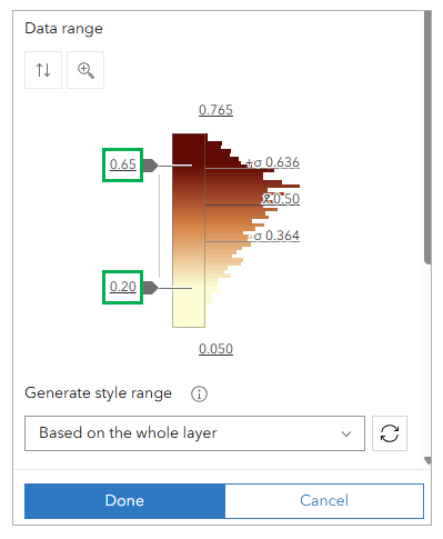
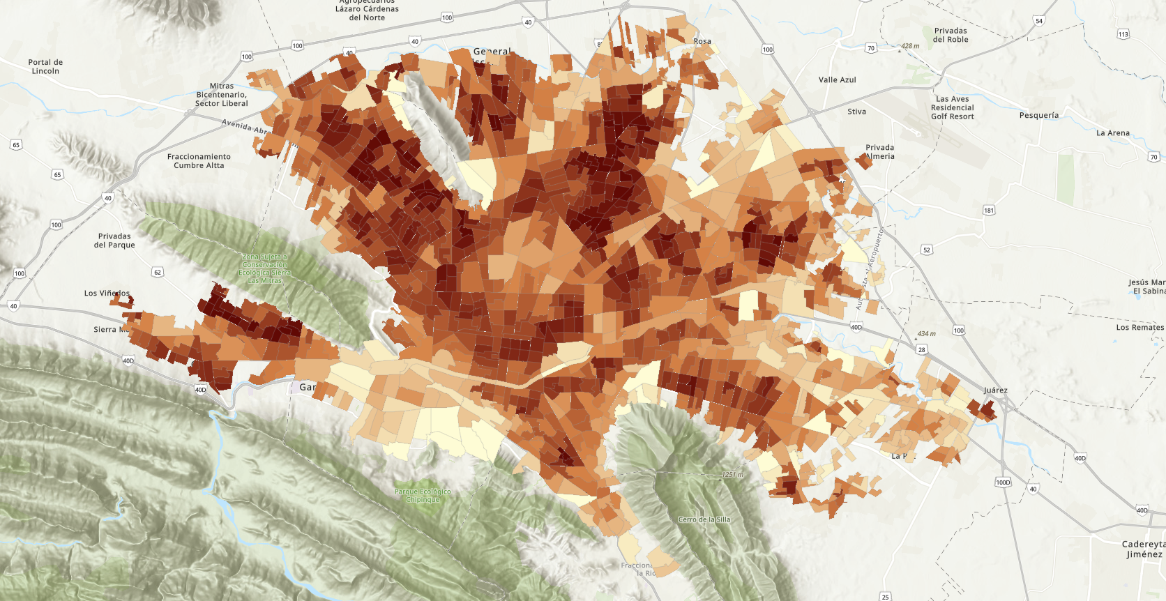
The data should now be visualized in a more striking red color ramp that better represents heat risk. You can change the visualization range to give it more clarity as well. In the Style options pane, find the Data range section. Click on the upper limit and type in “0.65”, then click on the lower limit and type in “0.2”. After the range has been adjusted, click Done.

You can now assess the data and determine what areas of Monterrey have the highest heat risk, and where heat island reduction efforts should be concentrated.