
We often aggregate points into bins in a grid to understand spatial patterns. But the bin size we select plays an important role in the resulting maps and the stories they tell. The same point data can tell very different stories at different aggregation scales.

This is often described as part of the Modifiable Areal Unit Problem (MAUP); a problem we often warn about but seldomly give tools to help with!
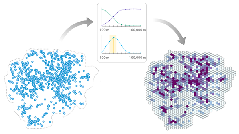
So how do we select an appropriate bin size?
The Evaluate Bin Sizes for Point Aggregation tool was released to help bring confidence to this decision. By testing a series of bin sizes, the tool finds bins that balance summarizing enough while still preserving the spatial point patterns in the data.

However, this raises new questions:
- What bin size should I use if points come with timestamps?
- What bin size should I use if points come with values of interest?
In ArcGIS Pro 3.7, the tool now supports two enhancements to help with these questions. Let’s see how these work.
What bin size should I use if points come with timestamps?
When points have timestamps, you can create spatiotemporal bins to analyze trends and create forecasts. But the same challenges described in the MAUP play a part when considering time: the bin size determines the trends we find and the forecasts we would create.
So, what bin size should we use?
You can now use the Time Field and Time Interval parameters to find bin sizes that properly account for sparser patterns when the data occurs in time intervals. For example:
- You want to analyze weekly trends of 311 service requests across the city.
- You set the Time Field parameter to the field containing the date and time of the request.
- You set the Time Interval parameter to 1 week.
- The tool splits the request points into weekly intervals before finding appropriate bin sizes.

The output layer is time-enabled and includes a set of features for each time interval, so you can see the aggregation patterns change over time.

The resulting bin size can be used as the bin size for the Create Space Time Cube by Aggregating Points tool before continuing on with your analysis.

What bin size should I use if points come with values of interest?
Points often have values that we need to analyze, and we can also aggregate point values to bins on a grid. For example, instead of just looking at restaurant point locations, you analyze the average sales revenue for restaurant point locations across each bin.
We face similar MAUP challenges when aggregating values, but there’s a new consideration: a bin mean is only a good representation of an area if the point values are not drastically different from the mean. As bin sizes get larger and larger, the mean often becomes a poorer representation of the area inside.
So how do we find a bin size that summarizes just enough before we lose too much information?
You can now set an Analysis Field, allowing the tool’s bin size recommendation to be driven by averaged attribute values instead of point counts.

This is useful for cases where the value itself is the focus – such as business sales revenue, pollutant concentrations, or incident response times – and where you want the chosen bin size to prioritize preserving spatial patterns of those values. When using an Analysis Field, you can choose between combining coincident points (averaging the values of collocated points and treating them as a single point) or handling the points separately.

At the end of the day, choosing a bin size is still an analytical decision. But with the Evaluate Bin Sizes for Point Aggregation tool, you can make a more informed decision by better understanding how scale affects your data. Whether you’re evaluating point counts, analysis field values, or either of these across time, the tool can guide you toward bin sizes that balance preserving spatial patterns with summarization. We encourage you to try out these new capabilities with your own data to see how thoughtful aggregation choices can support, rather than obscure, the stories your data are telling.
Resources
- Evaluate Bin Sizes for Point Aggregation
- How Evaluate Bin Sizes for Point Aggregation works
- Ramos, Rafael G. 2025. “Finding an Adequate Areal Unit to Map Crime: A Spatial Data Perspective.” New Research in Crime Modeling and Mapping Using Geospatial Technologies (pp. 27-44). Cham: Springer Nature Switzerland. https://doi.org/10.1007/978-3-031-81580-5_2.


Article Discussion: