Ever since the iNaturalist observations were made available in ArcGIS Living Atlas, we’ve visualized the data countless times using Map Viewer to support our storytelling about the natural world. From prairie dogs to coyotes and red foxes, our projects frequently feature this dataset, partly due to our fascination with nature but also because of its incredible extent and richness.

In Bog wild, we use the iNaturalist observations to explore the wild world of bogs in North America and the incredible plants that call these habitats home. This blog outlines some of the tips and tricks we’ve learned along the way for working with the data in Map Viewer and weaving these biodiversity maps into the narrative of our stories.

Techniques

As mentioned, the iNaturalist observations are extensive. The dataset contains millions of observations spanning nearly 500 species, so effectively wrangling and visualizing this data is essential to the story.

Filtering the data

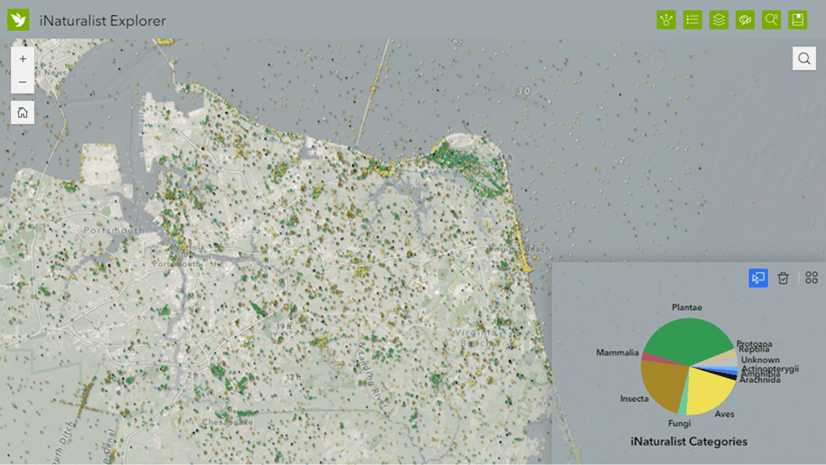
The prepared layers in the Living Atlas are great examples of how we can visualize the data at various scales using hexbins and the predominant size and category. This style shows the total number of observations within each bin and the most frequently observed taxon.

While convenient, the Living Atlas layers’ aggregation level wasn’t granular enough for us to explore each genus of carnivorous plant we hoped to map. We’d need to start from scratch with the individual observations.

Each observation in iNaturalist contains attributes such as species, location, time of day, and often a photo. This information contributes to the dataset being a reliable and invaluable source for scientists. It also allowed us to filter the observations to the five carnivorous plant genera we wanted to map in our story.

Aggregation

In mapping the observations of each plant throughout the story, we used aggregated hex bins to help with performance and visualizing the count of observations that would otherwise be difficult to discern from a mass of point symbols.

The process for creating our aggregation of carnivorous plant observations involved:

• Generating a tesselation of hexagons to serve as the bins to aggregate the observations from iNaturalist. You could also use one of the many existing hexbin layers in the Living Atlas or skip this step and use a bin layer created by the Summarize Within tool, one of the many geoprocessing tools available in Map Viewer.
• Then, using summarize within the carnivorous plant observations, we counted the observations of each plant genus within each hexbin.
• Joining these summary statistics back to the hexbins yields a column with a count of observations for each of our carnivorous plants inside that hexbin.

We selected the predominant category and size style to visualize this layer using the calculated summary count attributes.

Changing focus

When telling stories with geographic data, there are times when your map layers should demand attention and step to the forefront and other times when they should be supporting characters in the background. The cartographic choices you make when styling these layers can tailor them to their role in your story. Here are some ways to achieve subtlety or focus with your map layers.

Blurring boundaries

In Bog wild, we use the observations of carnivorous plants from iNaturalist to reveal the underlying bog habitat. We visualized this emergent pattern of bog habitat using the aggregated hexbins and incrementally including those where each plant genus was observed. However, bogs are complex ecosystems, and neither the iNaturalist observations nor our aggregated hexbins accurately captured their true extent. So, we softened their appearance using map effects and sketch layers as a mask.

• Create a Sketch layer, or use the Global background layer from Living Atlas and give it your choice of fill. We chose the dependable R Dot Fill 1 from the hatch fill category and set the marker position to random.
• Stacking this layer alongside the aggregated hexbins with a group layer we then applied the destination in blend mode. This handy technique is like a cookie cutter and cuts out the textured fill layer configured in step 1, where it coincides with the aggregated hexbins.
• To soften the edges of our cookie cutter, a blur effect was applied to the hexbins. This created a nice soft gradient hinting at unknown or undefined boundaries between the observed bog habitat and the surrounding area.

These textured layers with fuzzy or blurred edges can reduce the implied accuracy and precision inherent in GIS data. In addition, the organic pattern fills further enhanced this effect and had the added benefit of giving the layer some subtlety and pushing it to the background, yielding center stage for the hexbins with proportional symbols.

Create vignettes in Map Viewer →

Drawing attention

Inversely, there are times when we want to guide our readers through the maps in our stories, drawing attention to specific features or locations. In Bog wild, this meant directing the focus of our readers to specific bog habitats in North America. To achieve this, we used animated symbols, a recent addition to Map Viewer, to create pulsing location markers to direct the eyes of our readers to specific bogs of interest.

The hint of movement catches the eye and guides the reader to where we’d like them to look. When applied strategically, this effect can help lead your audience through the map, directing their attention to features and locations relevant to your story.

Use animated symbols in Map Viewer →

Finishing touches

Altogether, these techniques help to elevate the effectiveness of the map within the Bog wild story. Data wrangling and visualization enabled greater performance and succinct data visualization, while thoughtful cartography helped to emphasize layers of importance and direct the reader’s attention. Try these workflows out when creating your own story with iNaturalist data, and be sure to share. We’d love to see how you’re using this incredible dataset to create your own biodiversity stories.