Transforming Raster Data with Continuous Functions in ArcGIS Pro

In suitability modeling and multicriteria decision analysis, one common reason for inaccurate results is having inconsistent transformations. Input raster criteria often come in different units, different value ranges, and even opposite preference directions. If you combine them without first transforming to a common scale, the raster with the largest numeric range can dominate the output, regardless of its true importance. Correctly transforming the rasters is essential—it ensures that each criterion contributes appropriately and supports the goals of the analysis.

In ArcGIS Pro, you can apply transformations using various geoprocessing tools in the Reclass toolset with the Spatial Analyst extension. While several tools can transform raster values, many of them produce discrete integer output. The Rescale by Function tool addresses this by using continuous mathematical functions to transform input values, allowing output values to vary smoothly across the range of the data.

This blog explains how Rescale by Function differs from the Reclassify tool, shows how to transform raster data by applying different functions, and demonstrates how to choose the right function through a flood vulnerability example. It also introduces that the same capability is available within the Suitability Modeler, where the relationship between input values and transformed values can be visualized more clearly.

Rescale by Function and Reclassify

The Reclass toolset provides multiple geoprocessing tools to transform raster values. Two commonly used tools are Reclassify and Rescale by Function. They can both map an input range to a target output scale, such as to a suitability scale, but they behave differently.

The Reclassify tool performs a one-to-one mapping for categorical data such as land use types. It also assigns ranges of input values to fixed output classes, producing a stepped result with abrupt changes at class boundaries. For example, if an elevation raster is to be divided into fixed ranges such as 0–120 meters, 120–240 meters, and so forth, each with a different suitability score, Reclassify is the right tool to use. As a result, once the elevation crosses the 120-meter threshold, the suitability value jumps to the next class. In the reclassified output, notice how the elevation values are grouped into 5 distinct groups.

In contrast, the Rescale by Function tool uses continuous functions to transform input values, creating a smooth output that better represents gradual changes in suitability or preference. For an elevation raster, the suitability value changes continuously from location to location rather than jumping at predefined class boundaries.  In the rescaled output, the output is a surface of continuous values.

The following sections will guide you through the process for choosing and applying the appropriate transformation function.

How to use the Rescale by Function tool

Suppose you want to transform a distance to powerline raster into a 1–10 suitability scale for a solar farm siting model, where locations closer to existing power lines are more suitable since you can get the power onto the grid with less expense. A linear function is a good choice when the suitability decreases at a constant rate as the distances increase.

In the Rescale by Function geoprocessing tool:

1. Select the Dist_to_Powerline raster as the Input raster.
2. Specify the output raster name.
3. Choose Linear as the Transformation function parameter value.
4. Set the individual function parameters to fine-tune the function curve. For more information, see how the parameters affect the function.
   For the Linear function, the Minimum and Maximum parameters are automatically populated with the minimum and maximum values of the input raster. In this example, those values are 0 and 15000, respectively.
5. Define the lower and upper distance to powerline thresholds to determine the value range for the transformation. Assign scores to values outside these thresholds. For more information, see the interaction of the lower and upper threshold on the output values.
   In this example, the Lower threshold is set to 2,000 and the Upper threshold to 10,000, so the linear transformation is applied only within that range. Values below 2,000 are assigned to 10, which is the value in the Value below threshold parameter. The Value above threshold parameter defines that any input values above 10,000 are assigned to 1 in the output.
6. Set the output scale by entering 10 for the From scale parameter value and 1 for the To scale parameter value. This will cause closer distances to receive higher suitability values and farther distances to receive lower values.
   Note: By default, the Linear function increases in suitability with distance. However, in our case, the farther locations are less preferred; therefore, we will invert the function by reversing the default values of From scale and To scale parameter values.
7. Run the tool.

The tool applies the Linear function within the defined thresholds of 2,000–10,000, and transforms the resulting values to the specified evaluation scale 1–10. This produces a continuous output raster suitable for the solar farm model. The function on the right side of the figure shows how input values are transformed into final values.

How to choose a transformation function

The Rescale by Function tool provides thirteen mathematical functions for transforming input raster values to an output scale. Choosing the right function is important since it will dictate what the results of the analysis will be. For instance, if you are transforming criteria to a common scale to be used in a suitability model, it is critical to capture how the subject is responding to each input value.

A decision-tree diagram can help make the right choice.

The first question is whether the relationship between the input raster values and the transformed values is linear or not. A linear relationship means the transformed value changes at a constant rate as the input value changes.

The next question is how the transformed value changes as the input values change.

• In some cases, transformed values increase as input values increase. For example, in a winery site selection model, areas with greater solar radiation may always be more suitable.
• In other cases, transformed values decrease as input values increase, such as when a shorter distance to infrastructure is preferred.
• Other scenarios address where the relationship is neither increasing nor decreasing throughout the full range. Instead, mid-range values may be most suitable, while values at both low and high ends are less suitable. In those cases, a bell-shaped or other peak-type function is more appropriate.

The plots on the right illustrate how transformed values (y-axis) change with input raster values (x-axis). The shape of each curve helps you select a function by showing whether the change is constant or nonlinear, and whether the transformed values increase, decrease, or peak at a specified value. More details and examples for each function are available in The transformation functions available for Rescale by Function.

Example

The following is a simplified example of using the above guide in a flood vulnerability model. Each variable is transformed based on how it relates to flood vulnerability:

• Population Density:
  • Linear–No. Flood risk does not increase at a constant rate as population density increases.
  • Preference direction–Increase. Higher population density corresponds to higher flood vulnerability.
  • Function–Logarithm. This is appropriate when transformed values increase rapidly at lower input values and then level off as input values continue to increase.
• Impervious Surface Ratio:
  • Linear–No. Flood risk does not increase at a constant rate as the impervious surface ratio increases.
  • Preference direction–Increase. Higher impervious surface ratios correspond to higher flood vulnerability.
  • Function–Large or Logistic Growth. These are appropriate when transformed values increase slowly at first and then rise more rapidly as input values increase.
• Distance to Major Roads:
  • Linear–No. Flood vulnerability does not decrease at a constant rate as distance from major roads increases.
  • Preference direction–Decrease. Areas closer to major roads are more vulnerable, and vulnerability decreases as distance increases.
  • Function–MSSmall. This is appropriate when the transformed values initially remain favorable, then drop off sharply and before leveling off as input values continue to increase.

Transformation in Suitability Modeler

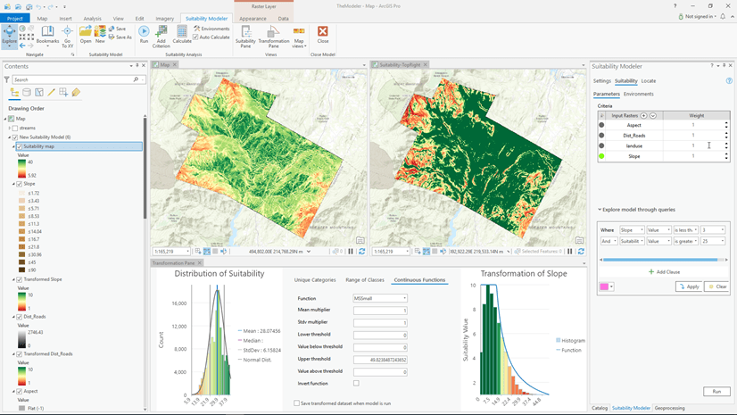
Use the Suitability Modeler to transform your data in a dynamic interactive environment. It uses maps, plots, and statistics to provide immediate feedback, helping you select the appropriate transformation methods and how to best refine their parameters.

After adding criteria in the Suitability tab, click the circular transformation icon next to a criterion to open the Transformation pane. The transformation plot displayed on the right shows the relationship between the input criterion and the transformed values. By choosing a function and adjusting the parameters, you can see how:

• The criterion values on the x-axis and the suitability values on the y-axis.
• The curve (the blue line) shows how input values map to suitability values.
• The histogram shows how input values are distributed across the study area, with colors indicating higher (green bars) and lower (red bars) suitability.

This interactive view makes it much easier to justify why a specific function was chosen and why certain locations were assigned high or low suitability values.

Summary

Accurately transforming raster data is essential for multicriteria decision-making analysis. The Rescale by Function tool offers a set of built-in transformation functions and a collection of parameter settings that enable you to customize the transformation function to best fit your specific analytical objectives. When transforming the raster using a continuous function within the Suitability Modeler, these capabilities are further enhanced with an interactive visualization experience.

Discover the capabilities of the Rescale by Function tool with your raster data. Experiment with various transformation methods and fine-tune parameters to align with your analysis objectives. Experience how you can enhance the insights you can make with multicriteria decision-making.

Read more

• • How Rescale by Function works
  • Formulas for the transformation functions