Unleash the power of RasterCellIterator to perform custom raster analysis

If you’ve read through the Introducing the Raster Cell Iterator blog, you’ll be familiar with the basic concepts of the Raster Cell Iterator (RCI), a new ArcPy class added in ArcGIS Pro 2.5 in the Spatial Analyst module that allows you to iterate over raster cells, query and modify individual cell values.

In this blog, let’s explore how RCI can be used to customize your analysis on problems that cannot be easily solved using the existing out-of-the-box geoprocessing tool. In the first example, we will use RCI to create a new raster with a specific spatial pattern – checkerboard. And in two other examples, we will use RCI to customize two focal operations: 1) count the number of neighboring cells that have a different value from the center cell, and 2) calculate the minimum slope from a DEM.

Create a new raster with the checkerboard pattern

In atmospheric modeling, a heterogenous surface raster represented by a checkerboard pattern can be used as an initial condition for idealized model simulations. However, there is not an existing geoprocessing tool with which you can create such a raster directly. In earlier ArcGIS releases, you can accomplish this task by using NumPy, but it would require a multi-step workflow to do so.  In ArcGIS Pro 2.5 with RCI, this task has become much easier! You simply need to assign a binary value to each cell based on the current row and column while iterating through a raster.  Following is a simple code sample which does exactly that.

 1
 2
 3
 4
 5
 6
 7
 8
 9
10
11
12
13
14
15
16
17
18
19
20
21
22
23
24
25
26
27
28
29
30
31
32
33
34
35

import json    
from arcpy.sa import RasterInfo, Raster  
  
# Create an empty RasterInfo object  
myRasterInfo = RasterInfo()  
  
# Load raster info from a Python dictionary  
myRasterInfoData = {  
  'bandCount': 1,  
  'extent': {  
    'xmin': -107.0,  
    'ymin': 38.0,  
    'xmax': -104.0,  
    'ymax': 40.0,  
    'spatialReference': {'wkid': 4326},  
  },  
  'pixelSizeX': 0.01,  
  'pixelSizeY': 0.01,  
  'pixelType': 'U8',  
}  
	  
# Convert myRasterInfoData to a JSON string and load into myRasterInfo  
myRasterInfo.fromJSONString(json.dumps(myRasterInfoData))  
  
# Create a new Raster object based on myRasterInfo  
myRaster = Raster(myRasterInfo)  
  
for (r, c) in myRaster:   
    # Checkerboard with 10 pixels width  
    if r % 20 < 10 and c % 20 < 10 or r % 20 >= 10 and c % 20 >= 10:  
        myRaster[r, c] = 1  
    else:  
        myRaster[r, c] = 0

myRaster.save(r 'C:\output\checkerboard.tif')  

From the code snippet above, lines 8-23 show the steps to construct a RasterInfo object from scratch. Line 26 creates an empty raster based on the raster info specified in the previous step. Lines 28-33 show the main logic of creating a checkerboard pattern raster by assigning binary values to the cell based on the current row and column. An implicit way of using Raster Cell Iterator is demonstrated by calling a simple For loop to go through all the cells. Since there is only one raster involved in this analysis, you don’t need to create a RasterCellIterators object explicitly. It is recommended to follow this pattern when you are working with only one raster. Finally, at line 35, we are saving the output raster. Figure 1 shows the output raster with the checkerboard pattern.

Custom Focal Operations

Focal operations produce an output raster dataset in which the output value at each cell is a function of the input cell value at that location and its neighboring cell values. With RCI, you can customize these kinds of focal operations with more flexibility.

Count the number of neighboring cells that have a different value from the center cell

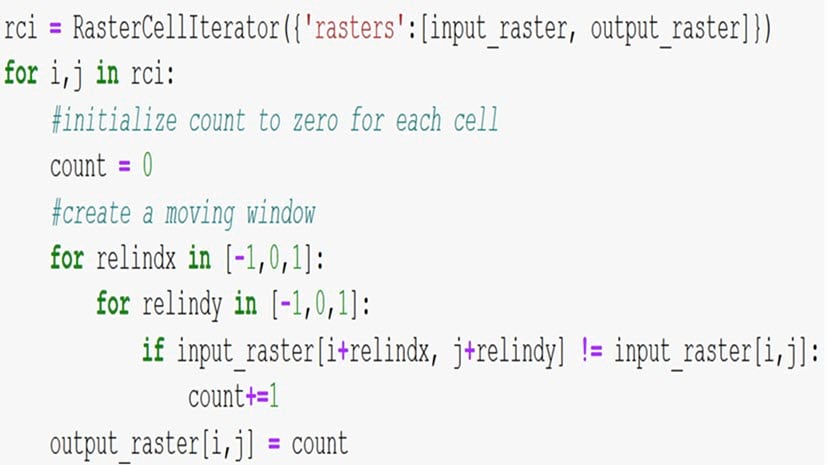
Stathakis & Tsilimigkas (2015) proposed several metrics to calculate the compactness of cities using land use adjacency information. To derive the compactness metric, one of the pre-processing steps is to iterate through the land use data and count the number of neighboring cells that have a value different to the center cell. This focal operation process is illustrated in Figure 2.

RCI makes it much easier to iterate over all cells and compare each cell value with its neighbors using a simple if logic. Here’s how you can do it yourself:

 1
 2
 3
 4
 5
 6
 7
 8
 9
10
11
12
13
14
15
16
17
18
19
20
21
22

from math import isnan    
from arcpy.sa import Raster, RasterCellIterator    
    
landu = Raster(r"C:\sample_data\landuse.tif")    
# Create a temporary output raster based on the raster info of landuse    
output = Raster(landu.getRasterInfo())    
   
with RasterCellIterator({'rasters':[landu, output]}) as rci:    
    for i,j in rci:    
        count = 0     
        # Assign NoData value to the output if the input is NoData    
        if isnan(landu[i,j]):    
            output[i,j] = math.nan    
            continue    
        # Create a moving window    
        for x in [-1,0,1]:    
            for y in [-1,0,1]:    
                # Count the number of adjacent cells with a different value      
                if not isnan(landu[i+x,j+y]) and landu[i+x,j+y] != landu[i,j]:    
                    count+=1    
        output[i,j] = count    
output.save(r"C:\output\landuse_diff_count.tif")   

In line 6, we are creating a new empty raster using the land use raster as an input template. Line 8 creates a RasterCellIterator object explicitly using input and output. In lines 9-21, we are looping through all cells in the input raster, and for each cell comparing its value to each of its immediate neighbors based on its relative position.

While performing the analysis, it is required to check for the NoData cells in the input, so that an appropriate value can be assigned to the output raster.  In lines 12 and 19, we are using isnan() function from the math module to check if the cell value in the input raster is NoData.  Line 13 uses nan from the same math module to represent NoData. In this example, NoData values are not considered while iterating through the cells and they are excluded from the neighbor cells when counting. The input land use data and the final output raster used in the sample code are shown in Figure 3.

Calculate minimum slope from a DEM

For the Slope geoprocessing tool, the slope value of each cell is determined by the rates of change of the elevation in the horizontal and vertical directions from the center cell (How slope works). In some cases, you might be interested in calculating the slope using a different equation. For an example, when building a fish trawlability model, an analyst might want to use a slope of the seabed that is based on the minimum change of elevation across each cell. By creating a custom focal operation with RCI, the following example shows how to calculate the minimum slope for your bathymetric DEM:

 1
 2
 3
 4
 5
 6
 7
 8
 9
10
11
12
13
14
15
16
17
18
19
20
21
22
23
24
25
26
27
28
29
30
31
32
33
34
35
36
37

from arcpy.sa import Raster, RasterCellIterator

dem = Raster(r'C:\sample_data\demtif.tif')
cell_x = dem.meanCellWidth
cell_y = dem.meanCellHeight
cell_diag = math.sqrt(cell_x**2+cell_y**2)
raster_info = dem.getRasterInfo()
neighbors = {
    # pixel offset: distance
    (-1,-1): cell_diag,
    (-1,0): cell_y,
    (-1,1): cell_diag,
    (0,-1): cell_x,
    (0,1): cell_x,
    (1,-1): cell_diag,
    (1,0): cell_y,
    (1,1): cell_diag
}
radian_to_degree = 180 / math.pi

# Set the output pixel type to be float 32 
raster_info.setPixelType('F32')
min_slope = Raster(raster_info)
with RasterCellIterator({'rasters':[dem, min_slope]}) as rci:
    for r,c in rci:
        slopes = []
        # Iterate through 8 neighbors to calculate the slope from center cell
        for x,y in neighbors:
            delta_y = abs(dem[r,c]-dem[r+x,c+y])
            # Calculate percent slope
            slope = delta_y / neighbors[(x,y)]
            # Calculate degree slope
            # slope = math.atan2(delta_y, neighbors[(x,y)]) * radian_to_degree
            slopes.append(slope)
        # Assign the minimum slope to the output cell value 
        min_slope[r,c] = min(slopes)
min_slope.save(r'C:\output\min_slope.tif')

In the code sample, lines 26-36 implement the main logic for calculating the minimum slope. For each cell from DEM, we iterate through its eight neighbors and calculate the rate of change. Then we find the minimum slope and assign that value to the output cell. Note that in line 22, the pixel type is set as ‘F32’, which means that the output is expected to be a 32-bit floating raster. In this example, the raster info of the slope output is inherited from the input DEM data. If the pixel type of your DEM data is integer, you need this step to make sure that the slope value of each cell is calculated as a floating-point value instead of an integer.

Summary

In this blog, we went through three different examples of using Raster Cell Iterator in ArcPy, each of them showing how easy it is to perform custom raster analysis. We hope you start using this simple but powerful capability to extend your own raster analysis capabilities.  Please let us know if you have any questions or want to see other examples and use cases.  You can also pass along any cool applications you come up with, and we can share your solutions with the community at large!

Reference:

Stathakis, D., & Tsilimigkas, G. (2015). Measuring the compactness of European medium-sized cities by spatial metrics based on fused data sets. International Journal of Image and Data Fusion, 6(1), 42-64.