
What are the most popular coffee shops near me? How many of these are less than five minutes away? These are classic GIS questions that can be answered using spatial analysis and transportation datasets. Similar techniques are employed when analyzing utility datasets, however, instead of locating the best cup of coffee, the focus is on reliability and customers:
- How is the customer being served by the network?
- What is the quality of the service the customer is receiving?
- If the customer’s service is interrupted, how can we reroute nearby resources to restore service?
Answering these questions requires knowledge of the path from the customer’s location in the network to a source (a feature that provides resources) or a sink (a feature that collects resources). Analysis then answers the question by measuring distance, counting equipment, or performing more advanced calculations along the path within the network.
In this article you will learn how to answer these types of questions using the tracing capabilities of a utility network. If you’re unfamiliar with tracing or ArcGIS Utility Network, you should read the introduction to the trace framework article first.
To get started, let’s look at extending an upstream trace.
Tracing and Functions
Running an upstream trace allows you to find the path towards any sources in your network, or in the case of a sink-based network it allows you to find all the paths heading away from the sinks in the network.
When running an upstream trace, we are often curious about what the journey from the starting point to the source upstream looks like. These questions typically ask for information such as “What is the distance from the starting location to the source? or, “How many devices are upstream of the starting location?”
These kinds of questions can be answered by adding the following functions to the trace configuration.
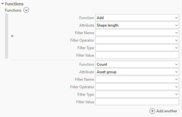
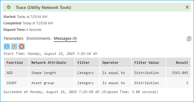
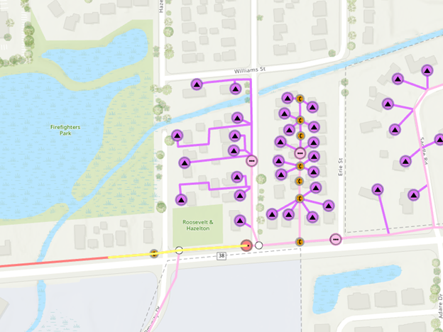
A function will apply a calculation to all the features returned by the trace and display them in the trace results. The Add function will add the Shape Length values for all the features in the results, giving us the total length of all the lines in the trace. The Count function will count how many features are in the path by relying on the fact that every network feature has an asset group that can be counted.
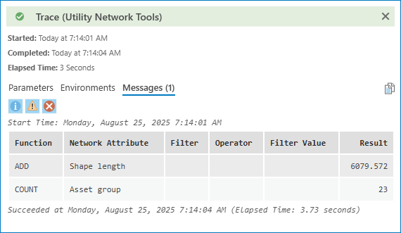
This results in the following values being returned by the trace shown above.
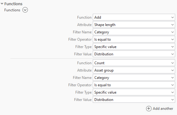
What if we wanted to limit the results to distribution equipment?
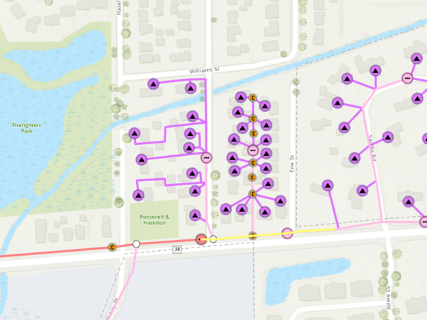
In that case we could use the filtering fields for each function to only calculate values that meet the filter criteria. In the example below we added a filter for features that have a custom network category called Distribution assigned to them.
After running the trace, we can see the results reflect the values of the upstream distribution features:
Functions are great for providing situational awareness, but what if you want to use them to control results? You will learn how to do that in the next section.
Stopping at a certain distance
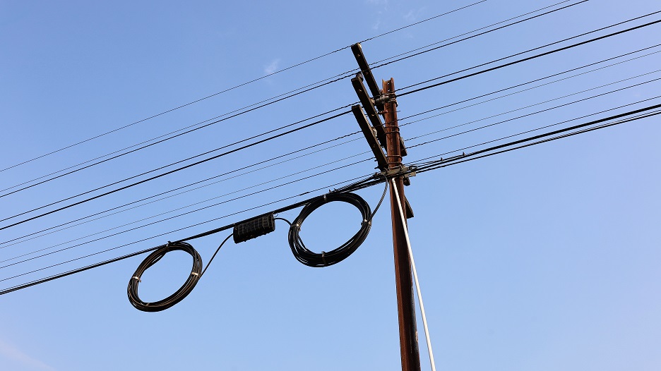
When troubleshooting connectivity in a fiber network, it is common for technicians to use a special tool called an OTDR (Optical Time Domain Reflectometer) to analyze and locate a fault. This piece of equipment uses a powerful laser to send a pulse into a fiber strand then measures the amount of time it takes light to reflect back to the device to calculate the distance and signal loss of the connection for that fiber. The ability for this analysis to identify the distance of the signal is what makes this tool invaluable for identifying faults or cable breaks.
The distance returned by the OTDR is the distance estimated based on the distance the signal traveled. The distance the signal travels does not always correlate to the horizontal distance travelled on a map. This is because the infrastructure supporting the signal is inherently 3D. Cables run up and down poles through risers, extra coils of cable are stored in slack loops, the poles themselves are placed on hillsides and mountains, and the heavy fiber optic cables can sag deeply between poles.
Knowing that a signal traveled 1500 feet before it encounters a fault is useful, but to fix the fault you need to be able to identify where in the physical world this is. In the previous section you saw how you can use a Function to calculate distance for a trace. Previous articles also demonstrate that we can use Barriers to stop a trace. To build on this, you can review the trace configuration for a utility network and see that there are two parameters which appear as if they can solve this problem:
- Function Barriers
- Filter Function Barriers
These two parameters are similar, but they each serve their own unique purpose.
Filter Function Barrier
A filter function barrier is best used with an upstream or downstream trace to identify the upstream or downstream features of the start point. The filter function barrier allows the source or sinks to be located, then limits the resulting features to meet the criteria you specified, such as stopping after a certain distance has been travelled.
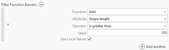
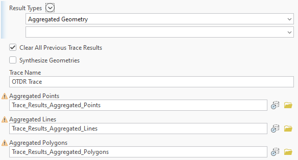
Because the trace is likely to stop in the middle of a line, we need to ensure we use the Aggregated Geometry result type. This ensures we return a geometry that represents the partial edge of the result, instead of selecting the entire feature.
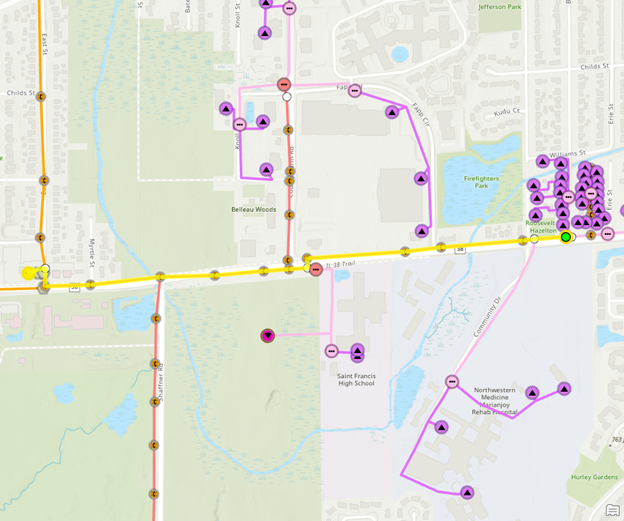
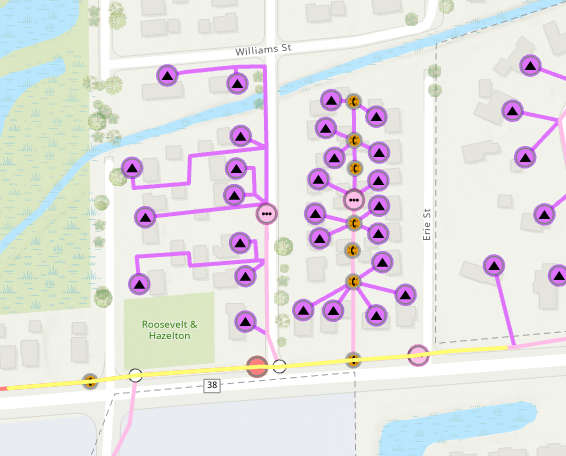
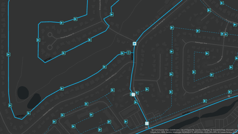
The trace result below (yellow line) now stops 500 feet upstream of the start point. This is the location where you can expect to find the fault.
If the fault is downstream of the current location (away from the central office), you would use the downstream trace to locate the fault. You can see the trace results below (yellow line) now show the location 500 feet downstream from the start point.
This result allows field crews to quickly identify the location of the fault in the field, providing knowledge not only of which cable they need to repair but also the location along the cable where the fault occurred.
Function Barrier
A function barrier is used to control when a trace stops, in utility network terminology this means that it is part of the conditions evaluated to determine traversability across features in the network. Function barriers are useful with a connected or shortest path trace, because you want the trace to stop once it meets the criteria of the function barrier and do not have the need to first identify the source or sink controllers. Using a function barrier with a subnetwork-based trace, like upstream or downstream trace, will often result in the trace failing because it can’t reach a subnetwork controller due to the defined function barrier.
Going back to the original example and running a connected trace with a 500-foot function barrier to create an aggregated geometry result.
Because you ran a connected trace, the trace result is returned both going towards and away from the central office (off-screen to the left). A connected trace isn’t aware of subnetwork controllers, so it considers paths on either end of the starting location. This is easily addressed by adding a barrier on the side of the device you don’t want to analyze.
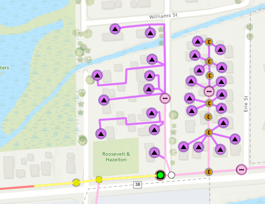
By adding a barrier on the downstream edge connected to the device (not visible underneath the start point) we can constrain the trace to show the upstream features. This is only required because the area being analyzed doesn’t have a source or sink to calculate flow, so we must manually orient the trace using a feature barrier.
Conclusion
In this article you learned how to perform calculations using a trace configuration. You saw how these functions can be used to present values or even constrain the results to specific conditions. The examples shown in this article were all based on a communications network, but similar equipment and techniques are used in pipe networks to identify blockages or electrical networks to identify faults.
Answering questions about what or how features in your GIS are connected is one of the fundamental capabilities of ArcGIS Utility Network. In earlier articles you learned the basics of the trace framework, how containers and associations can be used to answer questions, and even how to perform more complex analysis like isolation tracing. The main thing that all the previous examples have in common is they are trying to answer the question by using the topological relationships between features in the network to answer questions.
If you’re interested in watching a presentation that discusses these topics, you can find the Advanced Network Management (2024) presentation from the Esri User Conference on the Esri Video site
You can also visit the Esri Community site for ArcGIS Utility Network to ask any questions and see what others in your community are up to with tracing and analysis.

Commenting is not enabled for this article.