You sense a slight rocking and look up to see the leaves of the plant on your shelf sway almost imperceptibly. "Did you feel that?" you ask your office mates. No one did, so you link to the United States Geological Survey (USGS) Earthquake Hazards Program Web site to view a ShakeMap of the world's most recent earthquakes. You find that your area just experienced a magnitude 2.9 shaker, and smugly you announce this to your coworkers.

This is an example image of focal mechanism symbols created by 3D Focal Mechanisms near the epicenter of the magnitude 7.9 2002 Denali Fault earthquake. View is to the northeast. The junction between the Susitna Glacier Thrust Fault and Denali Fault is shown. There are numerous thrust-motion focal mechanism symbols in the region between the surface rupture of the Denali Fault and the arc of the Susitna Glacier Thrust Fault.

By the breadth of information and maps on the Web site, it is obvious USGS has been doing extensive research and monitoring of fault activity around the world. GIS has played a key role in USGS efforts of compiling, storing, processing, and serving earthquake information on the Web, which enables geologic scientists to visualize and understand the nature and instability of the ground on which we live.

Part of the USGS earthquake story includes the study of faults. When the earth's tectonic plates (part of the earth's crust) compress, they displace rocks on either side, which results in recognizable fault lines. When pressure builds, these sinuous threads of fault generate earthquakes, trigger landslides, and set off tsunamis. A great deal of data can be collected following an earthquake, such as its location, depth, magnitude, and amount of slip; the people it affected; and aftershock activity. USGS is constantly gathering fault data for analysis and modeling and then sharing its work with governments, scientists, and the public.

Peter Haeussler measures offset of the Susitna Glacier thrust fault.

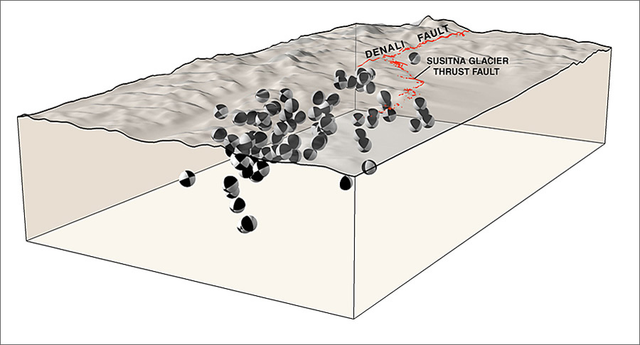
Geologists have been very interested in the central Alaska Range, which was formed by the Denali Fault system. They believe that the mountain chain was created by the tectonic collision of the Yakutat terrane, a "microplate," which has been colliding with Alaska for the last 10�20 million years. The Denali Fault is one of the longest strike-slip fault systems in the world and extends 1,200 kilometers from southeast to south-central Alaska.

The Alaska Earthquake Information Center is part of the nation's seismic monitoring network. The USGS' Alaskan outpost of its Earthquake Hazards Program in Anchorage works with the center, sharing research that is used nationally.

In 2002, the Denali Fault slipped, generating a magnitude 7.9 earthquake that ruptured 209 miles of the earth's surface. This was a strike-slip earthquake, where the ground moves side to side, a phenomenon that has produced earthquakes of this magnitude only a half dozen times worldwide in the last hundred years.

Peter Haeussler, the outpost's research geologist, is studying the Denali Fault, specifically, the fault's paleoseismology, to determine the ages when ancient earthquakes occurred along the fault. To do so, his geology team digs a trench across a fault area, records data, and maps the walls of the fault. This reveals strike, dip, and rake information that indicates the direction of a fault's movement. Most importantly, the studies show the timing of ancient earthquakes along the whole fault system. Using GIS, Haeussler created a map that shows where the fault ruptured in the 2002 earthquake, the width of the zone's area that was deformed by the slip, and how branching faults have come together.

Fault scarp near Augustan Creek, just west of Delta River. The offset was approximately 16 feet. Some cracks were up to 9 feet deep. A pressure ridge is visible in the background.

The Denali Fault earthquake was a complex rupture wherein three different faults were involved in the overall earthquake sequence. The ERDAS Stereo Analyst extension for ArcGIS proved very useful for understanding the event. Following the earthquake, researchers captured fault images from an airplane by using digital photogrammetry technology that included digital positioning data. This imagery data was then input into ArcGIS Desktop with Stereo Analyst. Haeussler viewed the data and denoted the small fault strands along the fault trace to create a three-dimensional map of the surface rupture of the fault.

"The technology helped me see features I ordinarily would have missed," explains Haeussler. "I was able to recognize patterns seeing, for example, how part of the thrust fault had rolled over and was heading downhill. I would have otherwise assumed it was vertical. It turns out it wasn't. I was able to see the fault was now actually dipping one way or the other, which helps me to better understand how the fault works. I could view the digitized vectors in ArcGIS 3D Analyst and rotate the image so I could view it from various angles."

Haeussler and his colleague Keith Labay also designed a tool for the ArcGIS 3D Analyst ArcScene application called 3D Focal Mechanisms (3DFM, available at pubs.usgs.gov/ds/2007/241). It allows the user to view earthquake focal-mechanism symbols three dimensionally. For example, the GIS geodatabase includes earthquake locations containing strike, dip, and rake values for a nodal plane of each earthquake. Other information, such as depth and magnitude of the earthquake, may also be included in the dataset. By default, for each focal point, 3DFM will create a black-and-white sphere or "beach ball" that is oriented based on the strike, dip, and rake values. If depth values for each earthquake are included, the focal symbol will also be placed at its appropriate location beneath the earth's surface.

Surface faulting split this tree near the Trans Alaska Pipeline.

This beach ball symbology is probably foreign to the layman. Basically, the beach balls show the direction and the slippage caused by the earthquake that occurred on the fault plane. A two-dimensional map that includes these diagrams does not reveal which plane actually moved in the earthquake, but by locating the symbols in 3D, image location becomes more apparent and can indicate the movement along a specific fault plane. The diagram's beach ball symbology may reveal similarity in clusters of the symbols' rotations that might suggest to a geologist that this is a particular kind of fault, evoking further investigation into complementary information surrounding that area.

In addition to the default settings, other options in 3DFM can also be adjusted. The appearance of the symbols can be changed by creating rings around the fault planes that are colored based on magnitude; showing only the fault planes instead of a sphere; drawing a flat disk that identifies the primary nodal plane; or displaying the null, pressure, and tension axes. The size of the symbols can be changed by adjusting their diameters, scaling them based on the magnitude of the earthquake, or scaling them by the estimated size of the rupture patch based on earthquake magnitude. It is also possible to filter the data using any combination of the strike, dip, rake, magnitude, depth, null axis plunge, pressure axis plunge, tension axis plunge, or fault-type values of the points. For a large dataset, these filters can be used to create different subsets of symbols. Symbols created by 3DFM are stored in graphics layers that appear in the ArcGIS 3D Analyst table of contents. Multiple graphics layers can be created and saved to preserve the output from different symbol options.

More Information

For more information, contact Peter Haeussler, geologist, USGS (e-mail: pheuslr@usgs.gov).