ArcUser Online

Time Approximate
Using multiyear estimates
By Lynn Wombold, Esri Chief Demographer

This article as a PDF .

The primary advantage of the American Community Survey (ACS) is that it supplies current data—annual estimates of the characteristics that were reported every 10 years from census sample data.

Since the full rollout of ACS in 2005, annual estimates have been reported every year, but only for areas with a population of 65,000 or more. Smaller areas require a pooled, multiyear sample to reduce the higher variance of their estimates. The first multiyear averages, 2005�2007, will be released at the end of 2008 for areas with a population of 20,000 to 65,000. In 2010, the first five-year average estimates, including all areas, will be released for the period 2005�2009.

What is the difference between a point estimate and a period estimate? With ACS, there is no conceptual difference. The annual estimates from the ACS are not point estimates, but pooled monthly surveys. Unlike the census, which represents a specific point in time (April 1), ACS is a rolling survey, a collection of monthly samples. The concept of collecting 36 or 60 monthly samples for the three- and five-year averages, respectively, is not very different from collecting 12 monthly samples.

However, the effects of minor operational differences for the data provider create a paradigm shift for the data user. There is a real difference between analyzing annual change and trying to interpret the change from multiyear averages. Annual ACS estimates do not appear very different from annual point estimates. The change from 2005 to 2006 can be calculated as a simple difference between the two years.

Since the U.S. Census Bureau also reports the margin of error, based on a 90 percent confidence interval, for each estimate from the ACS, you can determine whether the difference is statistically significant or not. It's an extra, although necessary, step in analyzing change, but the concept remains similar to assessing change in annual point estimates. The difference between 20,000 and 21,000 is still 1,000 or 5 percent. The only question with an ACS estimate is whether the difference is statistically significant or not.

When the two estimates represent multiyear averages, the question shifts from "what do the estimates reveal" to "what do the averages conceal." Suppose the estimate of 20,000 represents the period 2005�2007, and the estimate of 21,000 is an average of 2006�2008. The difference between 20,000 and 21,000 has not changed, but the estimates now represent three years, not one. The three-year periods, 2005�2007 and 2006�2008, also include two of the same years, 2006 and 2007. When the periods of multiyear averages overlap, the difference incorporates both the length of the multiyear period and the overlapping years.

By assuming that a multiyear estimate is simply the average of one-year estimates, the concept is easy to illustrate with a few examples. The examples in the accompanying tables are three very different patterns of change that yield exactly the same results in three-year averages. Keep in mind that the single-year averages are not reported for areas with a population less than 65,000. Only the three-year averages are revealed in ACS reports.

Averages with overlapping years show only a fraction of the real change in the estimates. These examples demonstrate the potential effect of two overlapping years in three-year averages. Only Example 2, which illustrates the result of a constant increase in the estimate, provides averages that are consistent with the annual trend. In Example 1, the sudden increase in the estimate in 2008 is minimized by overlapping averages. In Example 3, neither the precipitous decline in 2006 nor the significant increases in 2007 and 2008 are evident in the three-year averages. Changes in the overlapping years, 2006 and 2007, cancel out, which leaves only one-third of the difference between 2008 and 2005. If the estimate in question involves a specific population group, such as college students or retirees, the change can transform the characteristics of the area without warning.

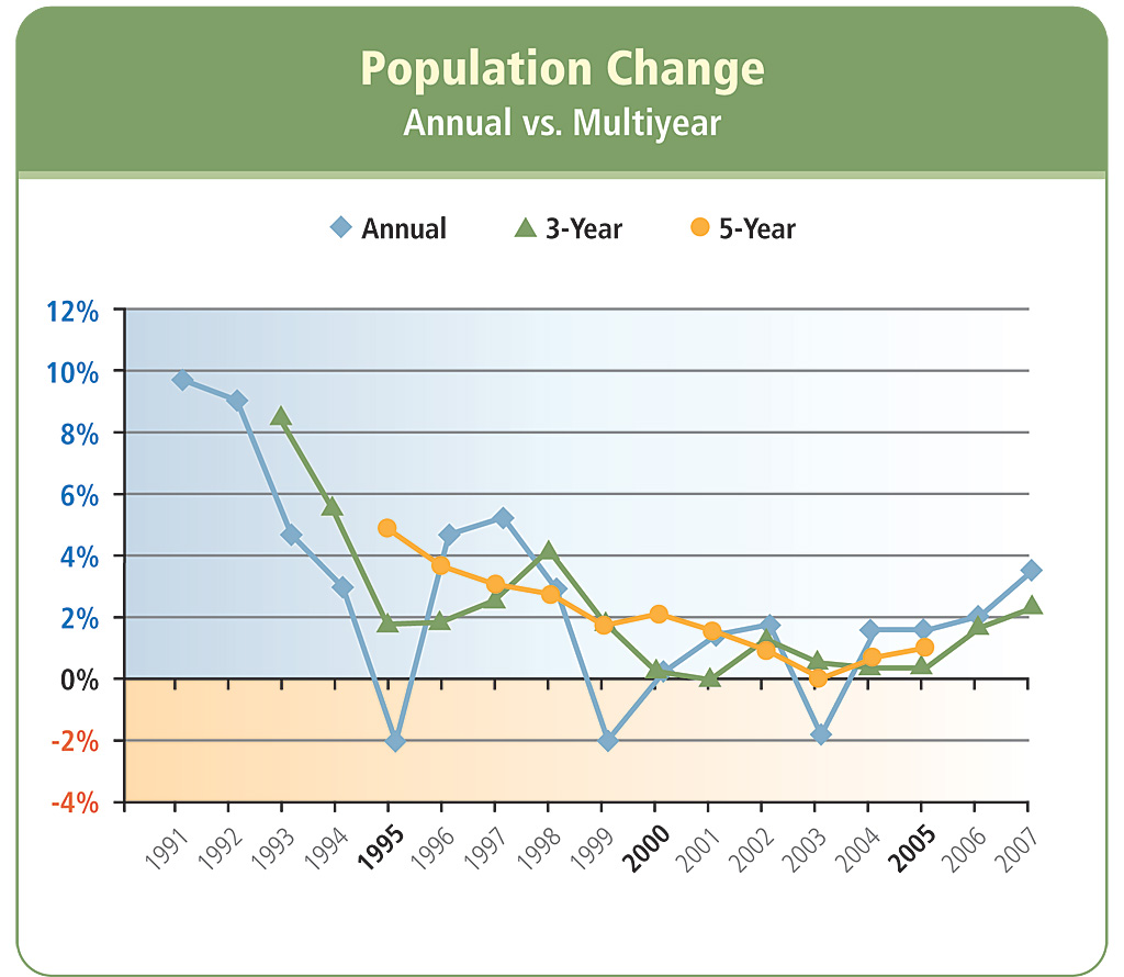
These examples may appear extreme. However, multiyear averages are to be used for the smallest areas, counties with populations less than 65,000 and subcounty areas such as tracts and block groups that are subject to extreme changes in population. Sudden growth from housing development is the most common change, but sudden loss of population due to the closing of a military base or factory or a natural disaster also happens. The graph in Figure 1 shows the variability of annual population trends that are calculated from point estimates and the leveling effect of three- and five-year averages. This county had a base population of 43,700 in 2000. The estimated changes in multiyear averages occasionally coincide with the annual estimates. However, obvious variations from the smoothed trend line are lost.

Significant shifts in the population are exactly the events that require current information about changes in demographic characteristics. Aggregate data from multiyear averages must be complemented by annual data on population change if the data user is to interpret the averages correctly.

If the understanding of multiyear estimates places this burden on the data user, why bother? The design of the ACS precludes any reporting of the sample data for small areas without multiyear averages. Pooling the monthly surveys to create a multiyear period estimate is necessary to reduce the variance of the sample estimates for small areas. The reduction in sample variance can only be viewed with data for areas that are large enough to support annual ACS estimates, but the effect is evident, even in larger areas. The table in Example 4 displays single-, three-, and five-year averages on median home value for Franklin County, Ohio. The base of this variable is owner-occupied units (259,142, +/-2,329), from the 2001-2005 ACS average.

The decrease in variance from one- to three- to five-year estimates is apparent; so is the "averaging" effect on median home value. In this example, the sample estimate increased at a steady rate from $121,500 in 2001 to $148,400 in 2005, about 5.5 percent annually. Therefore, the three- and five-year averages are at least consistent with the annual estimates. Unfortunately, this information will not be available for areas with a population less than 65,000. Only averages are to be reported from the pooled ACS samples. Although change can be tracked from each annual release of ACS data, estimates of change from overlapping multiyear averages are imprecise at best. If the one-year estimates are questionable for small areas, then one or two years of change in multiyear averages are equally uncertain.

Figure 1: Comparing annual and multiyear change in a county's population, 1990�2007.

Time is a specific reference point, even in the world of forecasts and estimates where data may represent a future point in time or incomplete information. The United States census has a designated Census Day, April 1 of years ending in zero. Current estimates commonly refer to July 1, a midyear point. Forecasts or projections represent a designated future date, usually July 1. These point estimates, or projections, enable simple calculation of change between two points in time. For data users who are accustomed to analyzing point data from a census, an estimate, or a forecast, the switch to a moving average is a reality shift. Current estimates of change are available from the ACS if you are willing to wait three to five (nonoverlapping) years.

Questions from readers are welcome. Please send them to lwombold@esri.com.

Other Articles in This Series

Three other articles by Lynn Wombold have been published on this subject in ArcUser magazine.

"Changes and Challenges—Understanding American Community Survey data." Oct.-Dec. 2007 issue of ArcUser

"Sample Size Matters—Caveats for users of ACS tabulations." Winter 2008 issue of ArcUser

"Examining Error—Consider the effect of sample size and error source when using census data." Spring 2008 issue of ArcUser

About the Author

Lynn Wombold, chief demographer at Esri, manages data development for Esri including the processing of census data and the development of unique databases, such as demographic forecasts, consumer spending, Retail MarketPlace, and the Community Tapestry market segmentation system, as well as the acquisition and integration of third-party data. She is also responsible for custom analysis and modeling projects. With more than 31 years of experience, her areas of expertise include population estimates and projections, state and local demography, census data, survey research, and consumer data. Prior to joining Esri, she worked for CACI Marketing Systems and was the senior demographer at the University of New Mexico. Wombold holds degrees in sociology with a specialty in demographic studies from Bowling Green State University in Ohio. She has received CACI's Eagle Award for Technical Excellence and Encore Achievers. The author of numerous articles for industry publications, she frequently presents papers on demography.