ArcUser
Summer 2012 Edition
Prospecting for Gold
Building, mapping, and charting point geochemical data
By Mike Price, Entrada/San Juan, Inc.
This article as a PDF.
This exercise uses a synthetic dataset developed from actual data that shows the location of anomalous gold occurrences in the Battle Mountain area of northern Nevada.
Data that has been imported from Microsoft Excel spreadsheets and geoenabled can be further explored using the charting capabilities in ArcGIS. To do this, the data points are first mapped as XY event themes, then imported into a geodatabase as feature classes.
This exercise teaches ArcGIS skills and workflows that are used daily by exploration geologists and geochemists. These skills include tabular joins, posting x,y point data using coordinates, thematic mapping, and statistical sampling. Once the data is mapped, the multielement charts, or scatterplots, available in ArcMap are used to identify and characterize the occurrences of these minerals.
"Importing Data from Excel Spreadsheets: Dos, don'ts, and updated procedures for ArcGIS 10" in the spring 2012 issue of ArcUser, defined a methodology for importing tables containing soil, rock, and stream sediment geochemistry into a geodatabase. Data tables included separate sample locations and metals analyses for soils and rocks, plus actual multielement data for stream sediments that had already been merged with locations.
Tip: Follow the file naming conventions carefully, and this exercise will be a breeze.
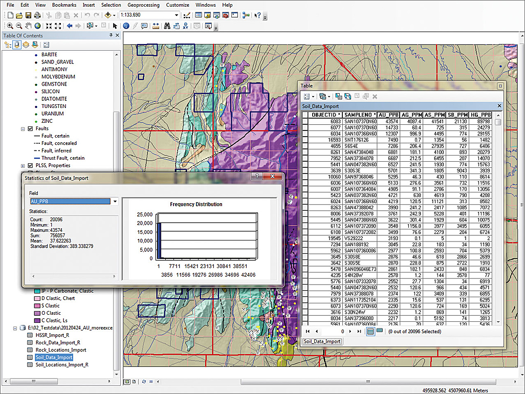
In the attribute table for Soil_Data_Import, choose Statistics from the context menu and characterize the data using a histogram.
This exercise uses a synthetic dataset developed from actual data that shows the location of anomalous gold occurrences in the Battle Mountain area of northern Nevada. Battle Mountain, a region of active mineral exploration and production, has been extensively prospected for more than 100 years. Geological and geochemical data is available through public sources. Exploration companies also maintain extensive private databases.
Getting Started: Exploring Battle Mountain
Although this exercise uses the same dataset as the previous tutorial, "Importing Data from Excel Spreadsheets: Dos, don'ts, and updated procedures for ArcGIS 10," it is best to start with a fresh copy of it. Before downloading this sample dataset for this exercise, archive any data you might have from the previous exercise.
Download the current training data and store it locally on your computer. Unzip the archive and explore the data in ArcCatalog. Preview the layer files. The Hydrogeochemical and Stream Sediment Reconnaissance (HSSR), Rock, and Soil data used in the previous exercise are not present. The first half of this exercise presents a workflow to build feature classes for this data so that it can be displayed.
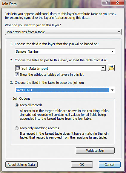
Join the Soil_Locations_Import_R and Soil_Data_Import tables. In the Join Data wizard, set item 1 to Sample_Number, item 2 to Soil_Data_Import, and item 3 to SAMPLENO.
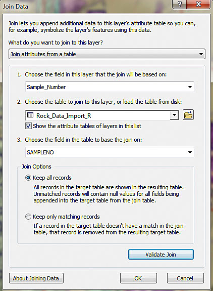
Join the Rock_Locations_Import and Rock_Data_Import_R tables. In the Join Data wizard, set item 1 to Sample_Number, item 2 to Rock_Data_Import_R, and item 3 to SAMPLENO.
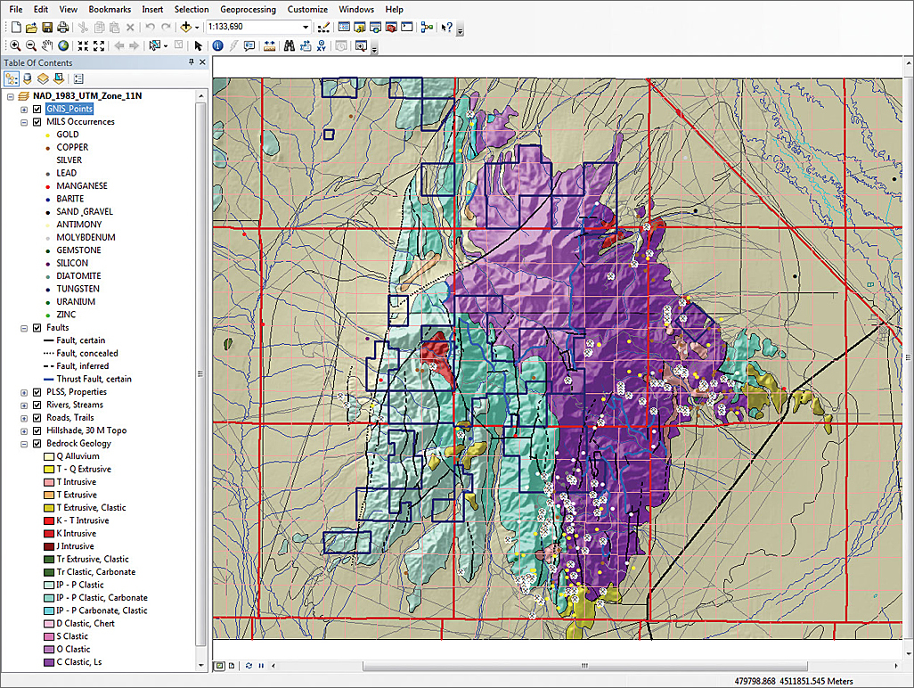
Close ArcCatalog and start a new ArcMap session. Navigate to \Battle_Mountain and open Battle_Mountain01.mxd. Explore the layers and become familiar with Battle Mountain geology. This region is characterized by Paleozoic sedimentary rocks that are more than 251 million years old. These rocks have been dislocated by extensive normal and thrust faulting. In many areas, older sediments occur above younger rocks—a geological oddity. Younger igneous rocks have intruded in the sediments, often bringing mineralizing fluids.
Battle Mountain includes many gold (Au), silver (Ag), and copper (Cu) mines and other mineral commodities, too. This exercise uses pathfinder elements in the synthetic dataset—arsenic (As), antimony (Sb), and mercury (Hg)—to guide the search for gold. Explore the US Bureau of Mines Mineral Industry Location System (MILS) points and compare the MILS commodities to the underlying geology. Check out the relationship between mines, prospects, lithology, and faulting.
Because HSSR_Import_R is in geographic rather than projected coordinates, set the coordinate system when creating the XY event theme by clicking the Edit button, then the Select button, and choosing North America > NAD83.prj.
Adding Geochemical Data
- Before loading the geochemical data into the map, turn off labels for the GNIS points. Click the Add Data button, navigate to \Battle_Mountain\GDBFiles\, and open the Geochemistry geodatabase. Select and load all five location and assay tables.
- As the tables load, ArcMap switches to the table of contents (TOC) Source tab so you can preview five geodatabase tables. Notice the location (Rock_Locations_Import and Soil_Locations_Import) and assay (Rock_Data_Import_R and Soil_Data_Import) data tables have identical record counts. Although this data has been carefully organized to enforce a one-to-one relationship between location and assay records, this is not always the case.
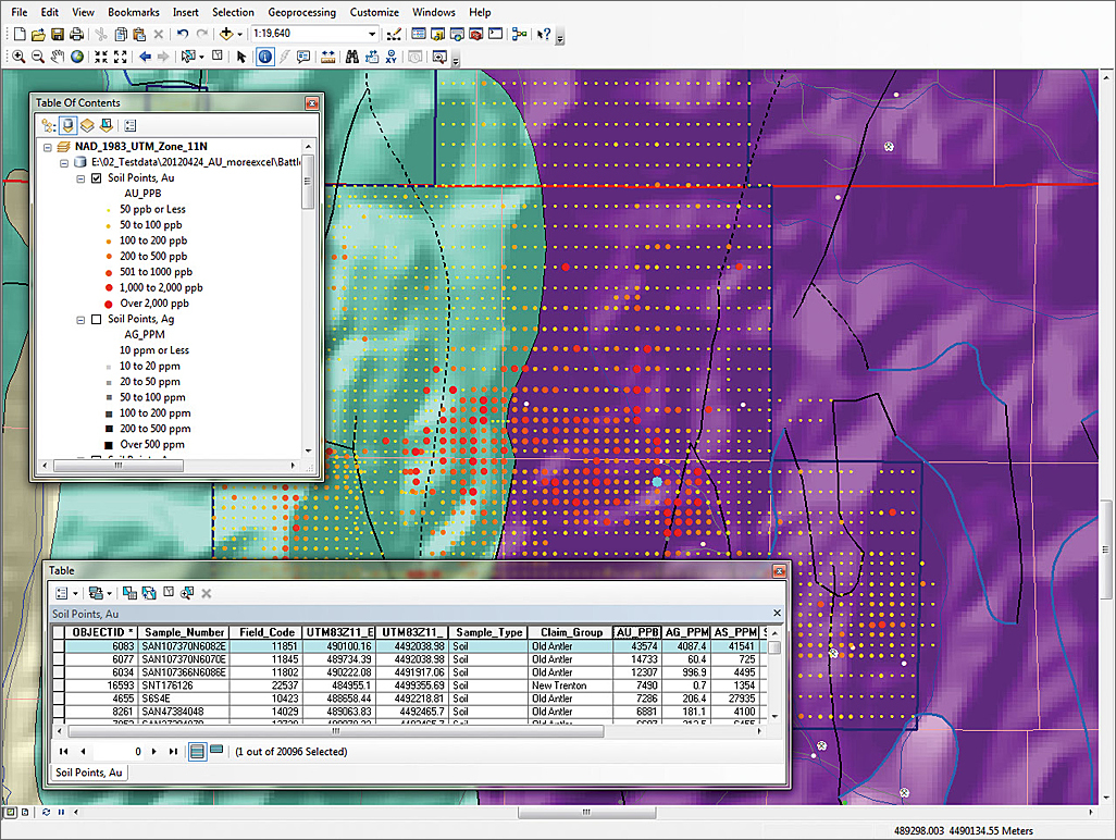
- Sort the soil assay data by element and right-click on the field containing the statistics for each element. Choose Statistics from the context menu to characterize the data using a histogram. The highest Au value is 43,574 part per billion (ppb), which equates to 1.40 troy ounces per short ton (i.e., the US ton, or 2,000 pounds). There must be a gold nugget in this sample.
- Inspect the HSSR and rock data. The rock samples are separated into location and assay files like the soil data. Rocks and soils data are both in universal transverse Mercator (UTM) North American Datum (NAD83) Zone 11 Meters, the same coordinate system as the map. HSSR coordinates are in NAD83 geographic (decimal degree) units. Explore the elements in these files using the Statistics tool. Remember that soil and rock data are both synthetic datasets, while HSSR points data is actual field data.
Joining and Exporting Soil and Rock Data
To place these datasets on the map will require joining and saving the soil and rock tables, exporting the joined table as a geodatabase table to preserve the short field names, and posting all three tables as XY event themes before exporting the XY theme to a geodatabase feature class.
- Process soil data first, then the rock data. Right-click Soil_Locations_Import_R and select Joins and Relates > Join.
- In the Join Data wizard, set item 1 to Sample_Number, item 2 to Soil_Data_Import, and item 3 to SAMPLENO. Click Validate to check the join, and click OK to complete the join. Sort the joined table as a second method of verifying that all records were successfully joined.
- Export this dataset to a new geodatabase table before posting it as an XY event theme. Exporting joined data first maintains the short field names in the final dataset, which is an important consideration. Right-click Soil_Locations_Import_R and choose Data > Export All Records to \Battle_Mountain\GDBFiles\Geochemistry.gdb. Name the table Soil_Data_Merge. Add the merged table into the map.
- Create a tabular join for Rock_Locations_Import and Rock_Data_Import_R. Inspect the join and export this table as Rock_Data_Merge.
- Open and inspect HSSR_Import_R. These coordinates are decimal degrees. Because these coordinates are already posted, a join is not necessary. Save the map.
After permanently saving the soil, rock, and HSSR points by exporting the XY Event themes to file geodatabase feature classes, they can be deleted from the map.
Mapping XY Event Themes and Saving XY Points as Feature Classes
Now to post soil, rock, and HSSR data as XY points. Once posted, each event theme will be saved as a geodatabase feature class.
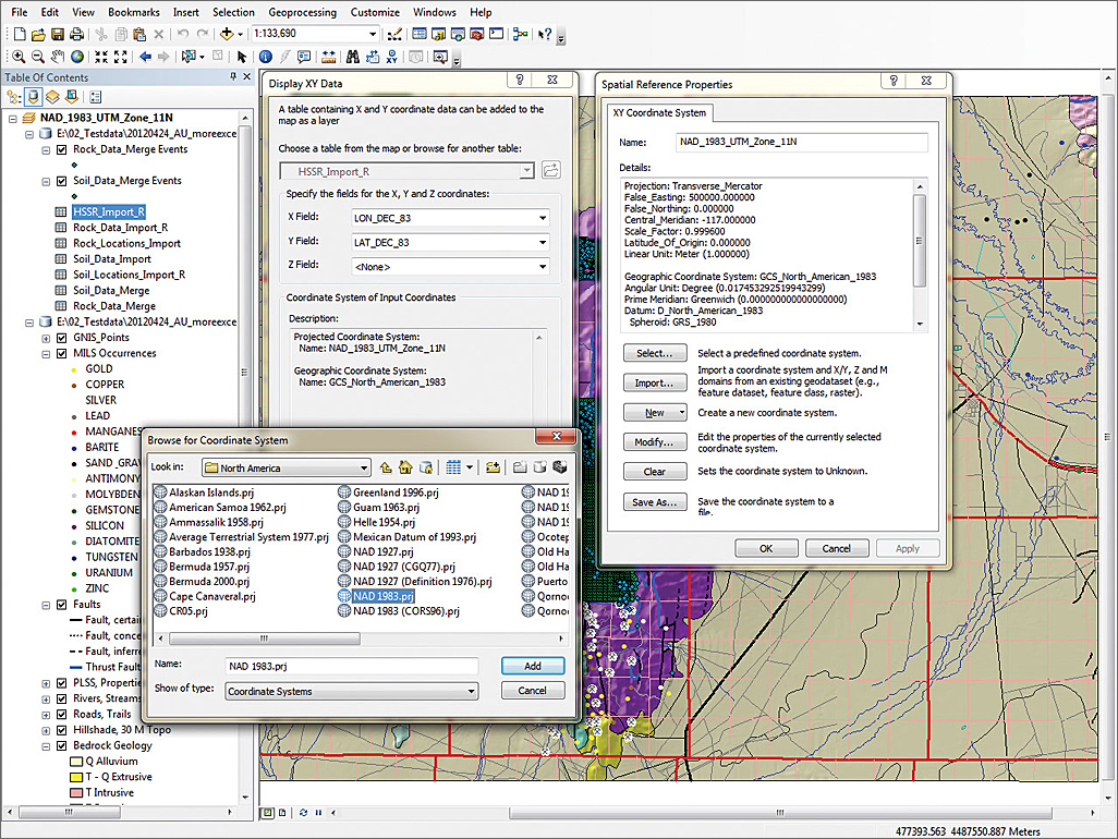
- In the TOC, right-click Soil_Data_Merge and select Display XY Data. In the Display XY Data wizard, set the X Field to UTM83z12_E and the Y Field to UTM83Z12_N and leave the Z Field as <None>. The predefined coordinate system should be NAD_1983_UTM_Zone_11N. If it is not, set it manually now by clicking the Edit button and using Select or Import.
- Click OK, and more than 29,000 soil points should appear on the map. Right-click Rock_Data_Merge and select Display XY Data. As before, set the X Field to UTM83Z12_E and the Y Field to UTM83Z12_N and leave the Z Field as <None>. The coordinate system should be predefined. Click OK to post Rock Points.
- Post the HSSR Points. Since HSSR_Import_R contains geographic rather than projected coordinates, the coordinate system must be carefully redefined. Change X Field to LON_DEC_83, Y Field to LAT_DEC_83, and Z Field to <None>. Click the Edit button to modify the coordinate system, then click Select and choose North America > NAD83.prj. Click Add, then OK twice. Save the project and inspect the new point sets.
- To permanently save the soils points, right-click Soil_Data_Merge Events and select Data > Export Data. Save the dataset as a file geodatabase feature class located in \Battle_Mountain\GDBFiles\Geochemistry.gdb. Name this feature class Soil_Points. Use exactly this file name. Add the new feature class to the map.
- After the Soil_Points layer appears in the TOC, export Rock_Data_Merge Events to \Battle_Mountain\GDBFiles\Geochemistry.gdb and name it Rock_Points.
- Export HSSR_Import_R Events to \Battle_Mountain\GDBFiles\Geochemistry.gdb as HSSR_Points. The point set is nearly completed. Save the file.
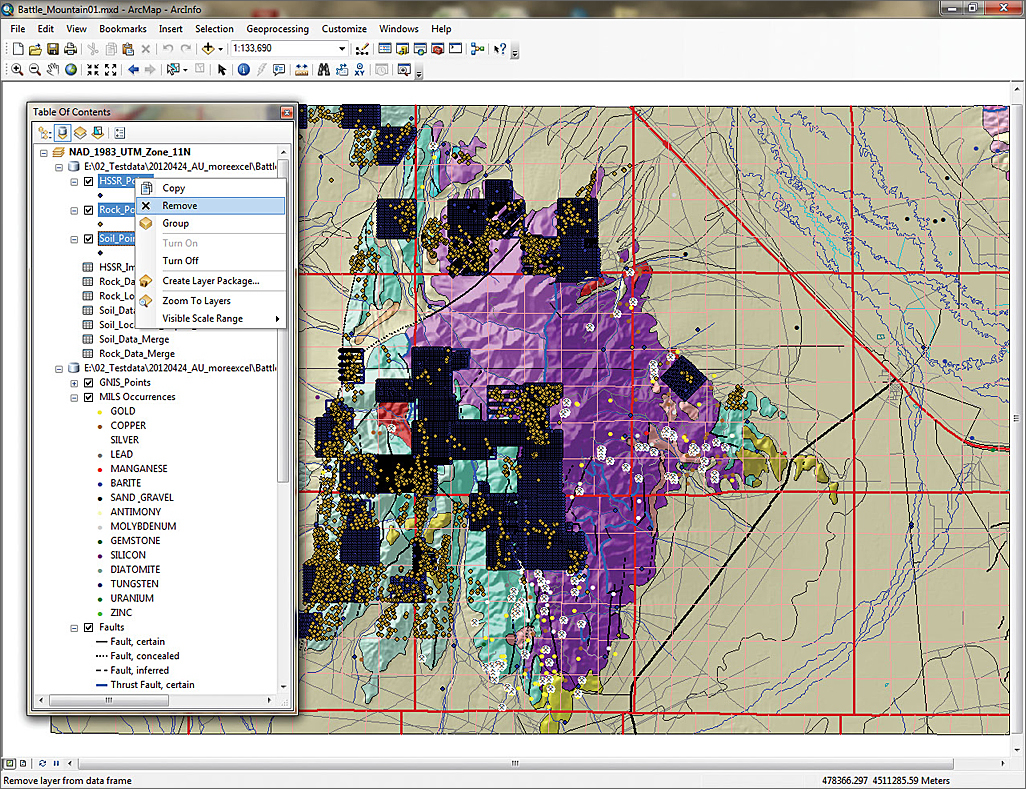
- Before continuing, simplify the project by removing the three XY event themes and deleting the two duplicated join fields (i.e., Soil_Points OBJECTID and SAMPLENO) in the tables for each new feature dataset.
- Also remove the three new geochemistry feature classes (Soil_Points, Rock_Points, and HSSR_Points) from the map. Save the map.
Now load the Soil Geochemistry Group, a set of layer files to symbolize the layers for Au, Ag, As, Sb, and Hg elements, and one layer each for Rock Points and HSSR Points.
Applying Prebuilt Geochemical Symbology
Remember the Soil, Rock, and HSSR layer files that could not be displayed properly when the map was opened initially? Now that the corresponding feature classes have been created, these layer files should load easily.
- On the text menu, select Bookmarks > Anomalous Soils 1:20,000 to zoom in to an interesting project area centered on Battle Mountain.
- Click Add Data and navigate to \Battle_Mountain\GDBFiles\. Select and load the Soil Geochemistry Group, seven point layer files that include five soil themes for the elements Au, Ag, As, Sb, and Hg, and one layer each for Rock_Points and HSSR_Points.
- If these files loaded properly, save the map again. If not, check the data paths and feature class names. You may need to rebuild data or change data pointers.
- Inspect all datasets and look for anomalous data. Notice that each layer file contains seven symbolized and colored data intervals separating high-grade points from background data.
- Notice the large red Au samples that appear above adjacent low-grade points. Symbol levels were applied to achieve this effect. Without symbol levels, many high-grade points would be covered by nearby low-grade samples, especially when shown at small scales. Symbol Levels changes the drawing order so low-grade points are drawn first and high-grade points are drawn last. To learn more about defining symbol levels, read the companion article, "Displaying Points: Using symbol levels to optimize point display."
The relationships between gold and other elements can be explored using scatterplot matrix charts.
Investigating Relationships Using a Scatterplot Matrix
In the Battle Mountain area, anomalous gold often occurs with elevated levels of silver, arsenic, antimony, and/or mercury. Using charting in ArcGIS, the relationships between the elements in the geochemistry data can be defined and plotted. In this exercise, XY scatterplots will be a quick and effective way to compare several elements. One chart will be created for each of five soil point element pairs for a total of 10 charts.
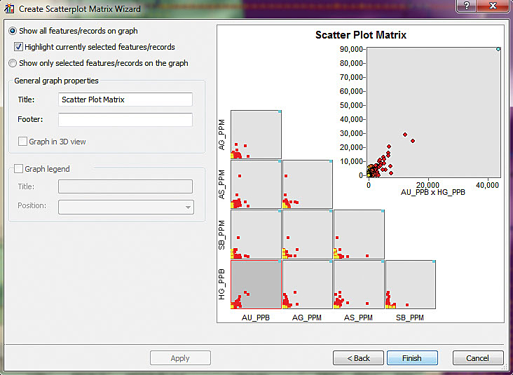
- On the ArcMap Standard menu, select View > Graphs > Create Scatterplot Matrix. In the Scatterplot Matrix wizard, set Soil Points, Au as the Layer/Table. Load all five assay fields in this order: AU_PPB, AG_PPM, AS_PPM, SB_PPM, and HG_PPB.
- Still in the same pane of the wizard, set the following parameters:
Color: Match with Layer
Brush Width: 3
Brush Height: 3
Style: Circle
Show Histograms: Unchecked (for now) - Click Apply, and 10 histograms should appear. Click Next and then Finish. Study the arrangement of the 10 scatterplots that evaluate the combinations of the five elements. Au/Hg should be the active plot. To switch plots, click the desired chart in the matrix, and it will appear in the active window.
- Right-click the largest, active plot to open Graph Properties. Preview the Series and Appearance tabs. Close this window. To display as much active mapping area as possible, dock the scatterplot window in the lower left corner of the display. If you have a dual monitor, move it to the other screen. Save the map again.
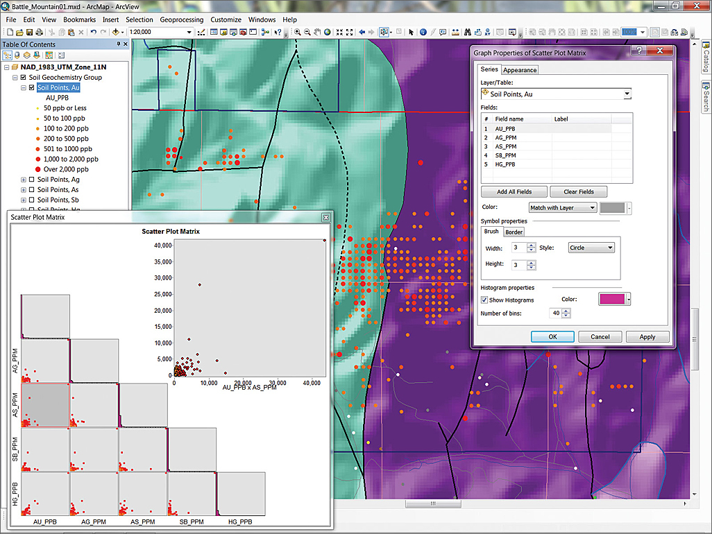
Right-click (or double-click) the active scatterplot, open Properties, and select the Series tab. Check the Show Histogram box, set the color to Peony Pink (a bright magenta shade), and set the number of bins to 40.
Let's Go Prospecting
One really useful thing about a chart in ArcGIS is that if you select data on a chart, the corresponding data will be selected on the map. You can also select vector data on the map and show the corresponding samples on each chart. These scatterplots show relationships between two elements, so we can chart them both, select interesting populations, and locate them on a map.
For example, with Au/Ag active, estimate the position of 5,000 ppb Au and draw a selection polygon to select all samples in the chart to the right of this Au value. (Hint: Select from lower left to upper right.) Be sure to catch the outlier in the upper right corner. Watch as the selected anomalous gold samples in the plot are highlighted on the map and in all 10 scatterplots. There are many anomalous samples in the area. Let's go check it out.
- On the Standard toolbar, select Bookmarks > Anomalous Soils 1:20,000. In the TOC, switch to the List by Selection tab and make only Soil Points, Au selectable. Select features by drawing a box around the largest group of red points in the center of the screen. These points will be highlighted on the map, in the selected scatterplot, and in each of the 10 scatterplot thumbnails.
- This next step creates a subset of moderate- to high-grade samples and shows distribution histograms for the five elements. Based on regional knowledge, any soil sample containing over 200 ppb Au is significant. (Remember, this is synthetic data provided for training purposes only.) Clear the selection set, and in the TOC, right-click Soil Points, Au and click Properties. Open the Definition Query tab, create a query to display only samples containing 200 or more ppb Au, and apply this query. The scatterplots will be redrawn showing only the anomalous samples.
- Right-click (or double-click) the active scatterplot, click Properties, and select the Series tab. Check the Show Histogram box, set the color to Peony Pink (a bright magenta shade), and set the number of bins to 40.
- Switch to the Appearance tab and click the radio button to Show only selected features/records on the graph. Click OK to apply the changes and create histograms for the anomalous subset.
- Here is another selection method. Because some of the highest-grade gold occurrences are closely related to high-angle normal faults, use Select By Location to select Soil Points, Au by proximity to faults. On the Selection tab of the TOC, click the Faults layer to make it selectable. Select all items except faults coded as Known thrust fault.
- From the standard menu, choose Selection > Select By Location. Set Soil Points, Au as the Target layer and Faults as the Source layer. Set Spatial Selection method to Target layer(s) features are within a distance of the Source layer feature. Apply a search distance of 300 feet and click OK. Save the map.
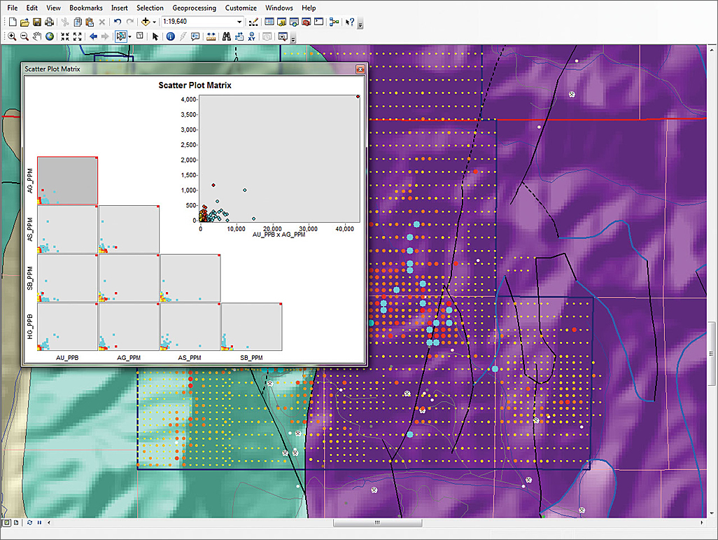
Estimate the position of 5,000 ppb Au on the scatterplot and draw a selection polygon on the active chart to select all samples to the right of this value. The selected samples will be displayed on the map and all scatterplots.
More Experimentation and Additional Training
This exercise experimented with only the large soil samples dataset. The sample dataset also contains more than 4,000 rock samples and almost 100 stream sediment points. You can continue evaluating these samples and study other proximity relationships including bedrock lithology and drainage systems.
To learn more about how GIS can be applied by exploration geologists and earth scientists, consider enrolling in Introduction to ArcGIS for Desktop for Mining Geoscience (IMIN), an Esri instructor-led course. It introduces ArcGIS tools to create mining geosciences workflows. Exercises teach fundamental ArcGIS skills and apply them to solve mining and geosciences problems such as detecting mineral occurrence patterns, locating prospective deposits, and identifying optimal areas for mineral exploration. Visit training.esri.com to learn more about this and other courses.
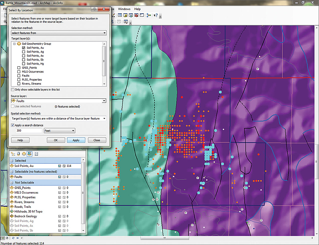
Because some of the highest-grade gold occurrences are closely related to high-angle normal faults, use Select By Location to select Soil Points, Au by proximity to faults.
Acknowledgments
The data in this exercise is essentially the same data presented in the spring 2011 ArcUser tutorial. While the soil and rock data is synthetic, it does match underlying geology. Landownership is imaginary, yet it reflects exploration trends around Battle Mountain, Nevada, in the early 1990s. Bedrock geology was derived from the Nevada Bureau of Mines and Geology county mapping series. HSSR data was developed by the US Department of Energy National Uranium Resource Evaluation (NURE) program. All data has been transformed from UTM NAD27 into the current NAD83 datum.