ArcUser
Spring 2012 Edition
Importing Data from Excel Spreadsheets
Dos, don'ts, and updated procedures for ArcGIS 10
By Mike Price, Entrada/San Juan, Inc.
This article as a PDF.
What You Will Need
- ArcGIS 10 for Desktop
- Microsoft Excel 2010/2007 or 2003 or the 2007 Office System Driver
- Sample dataset

This exercise models data from a well-known gold and base metals mining area in northern Nevada located near the town of Battle Mountain.
Many organizations keep valuable data in Microsoft Excel and comma-separated values (CSV) files. Learn a methodology for importing data kept in Excel and CSV files into ArcGIS that has been updated for ArcGIS 10 and Microsoft Office 2007/2010.
Excel spreadsheets have been used since the release of ArcGIS 8 to prepare and import tabular data into a GIS. Previous ArcUser articles described the benefits and limitations of spreadsheets in the version of ArcGIS current at that time. In early 2004, ArcUser editor Monica Pratt wrote "Working with Excel in ArcGIS." In 2007, the author wrote another article on the same topic, "Mapping and Modeling Groundwater Geochemistry."
Since these articles were published, Microsoft has released two new versions, Excel 2007 and Excel 2010. With each release, spreadsheet capabilities have improved and the processes for importing data into ArcGIS have changed. This article updates and refines rules and procedures for importing Excel 2003 files into ArcGIS 9.x.
Although the sample data is synthetic, it is true to the underlying geology of Battle Mountain, Nevada.
This exercise reexamines the Excel spreadsheet as a data import tool, focusing on ArcGIS 10 and Excel 2007/2010. The tutorial uses spreadsheets to create and enhance geologic data. Field samples include Hydrogeochemical Stream Sediment Reconnaissance (HSSR) points plus custom soil and rock data. In this exercise, we will model a well-known gold and base metals mining area in northern Nevada, located near the town of Battle Mountain. The custom samples are typical of data that might come from the field, assayed by a modern analytic laboratory.
A Word about Microsoft Excel Versions
If you have installed Office 2007, you can read .xls and .xlsx files. If you have Office 2003 or 2010 installed, you can read .xls files, but you will need to install the 2007 Office System Driver to read .xlsx files.
If you do not have Microsoft Excel installed, you must install the 2007 driver before you can use either .xls or .xlsx files. The 2007 Office System Driver can be downloaded from the Microsoft Download Center. Carefully follow the installation instructions before you restart ArcGIS.
Also, if you have previously specified on the File Types tab of the Customize > ArcCatalog Options dialog box that ArcCatalog show you .xls files, you'll need to remove this file type to be able to access Excel files directly.
Before beginning to work the exercise, read the accompanying article, "Best Practices When Using Excel Files with ArcGIS," for valuable tips on working with Excel data
Getting Started: Examining Files in ArcCatalog
Preview the sample data in ArcCatalog.
To begin this exercise, download the training data. Unzip the excelmagic.zip data into a project area on your local machine and start ArcCatalog.
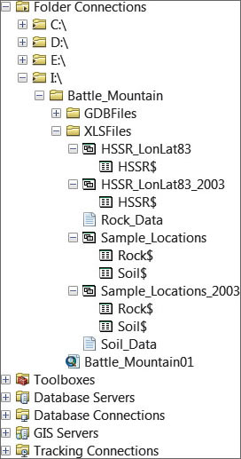
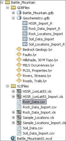
Navigate to the Battle_Mountain folder and locate the XLSFiles folder. When ArcCatalog displays an Excel file, it adds a dollar sign ($) to each worksheet name. Inside this folder, expand all files. Locate Sample_Locations.xlsx and preview Rock$. This Excel 2010 spreadsheet contains two worksheets named Rock$ and Soil$. Rock$ and Soil$ contain sample numbers, universal transverse Mercator (UTM) coordinates, and field information that allow this data to be posted on a map. Next, preview HSSR_LonLat83.xlsx and study its only worksheet, HSSR$.
Next, locate and preview two CSV files, Rock_Data and Soil_Data. These files contain companion analytic data for the Rock$ and Soil$ worksheets. The [SAMPLENO] field in both CSV files will support a one-to-one tabular join with the same field in the Soil$ and Rock$ worksheets.
Closely inspect the alignment of data in Soil_Data columns. Notice that [SAMPLENO] and [SB_PPM] are aligned on the left side of the column while [AU_PPB], [AG_PPM], [AS_PPM], and [HG_PPB] are aligned on the right. Scroll down through the table and observe that many fields in the right-aligned columns are empty. In the source CSV file, many of the fields contain nonnumeric strings that do not display properly.
Notice that [SB_PPM], a left-aligned field, contains many fields that begin with a less than (<) character. When a geochemical lab is unable to measure the presence of an element, the analytic posting will include a less than character, followed by the detection limit value. In [SB_PPM], the detection limit for antimony is five parts per million, and many samples contain less than this threshold value.
When ArcGIS reads an Excel worksheet table, it uses the first eight rows to define the field format. If those first eight rows contain mixed data types in a single field, that field will be converted to a string field, and the values contained in that field will be converted to strings. When ArcGIS reads a CSV file, the very first record defines the field type. Consequently, some rather detailed data preparation will be necessary before you can use these files. The next step will be to prepare the spreadsheet and CSV data for import into ArcGIS. Close ArcCatalog.
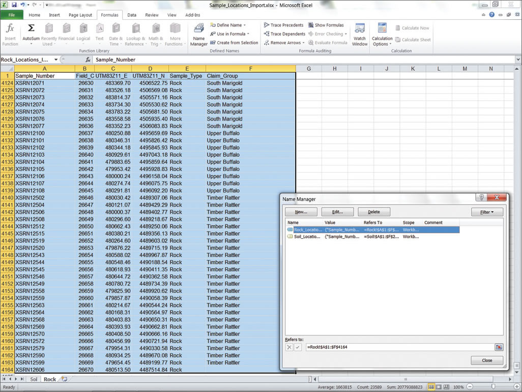
After field names have been corrected, create a named range in Excel called Rock_Locations_Import_R.
Preparing Excel Data for Importation
These detailed instructions are specifically for Excel 2007 and Excel 2010. If you want to try this exercise using Excel 2003, open Sample_Locations_2003.xls instead.
- Start Excel 2007 or 2010 and open \Battle_Mountain\XLSFiles\Sample_Locations.xlsx. Open the Soil worksheet and inspect the data. This location table contains 20,096 soil sample points, posted in UTM North American Datum 1983 (NAD83) Zone 11 Meters. Coordinates are posted and displayed using a precision of 0.01 meters. Many samples are coded by Claim Group.
- Save this spreadsheet as a new file so you can retain the original data as an archive. Name the new file Sample_Locations_Import.xls.
- Click the Soil$ worksheet and look at the first row of data. Many text strings in this row contain spaces. Change these spaces to underscores. (Hint: Select only the first row and use Find and Replace.)
- Next, clarify the coordinate system columns. Change Easting to UTM83Z11_E and Northing to UTM83Z11_N.
- Now define a named range. Move to cell A1. Notice that the titles are locked, so tap the F8 key to begin to extend a cell range. Hold down the Ctrl key and tap End to stretch the range (highlighted in cyan) to the lowest rightmost cell. Make sure the header fields are included in the highlighted area.
- In the Excel ribbon, select Formulas, click Name Manager, and click the New button. Name the new range Soil_Locations_Import_R. Click OK and close the Name Manager.
- Press the Ctrl and Home keys to return to the upper left live cell. Click the Name Box drop-down, located just above cell A1, to select and verify your range name. Save the spreadsheet file.
- Switch to the Rock$ worksheet and review this data. Make the same types of modifications to this worksheet to enforce correct field naming conventions. Make sure you have appropriate field names in the first row. (Hint: The tabular structure for the Soil$ and Rock$ worksheets is the same, so you can use the same procedure you used on Soil$.) Create a new range name called Rock_Locations_Import. Verify the new range and save the file.
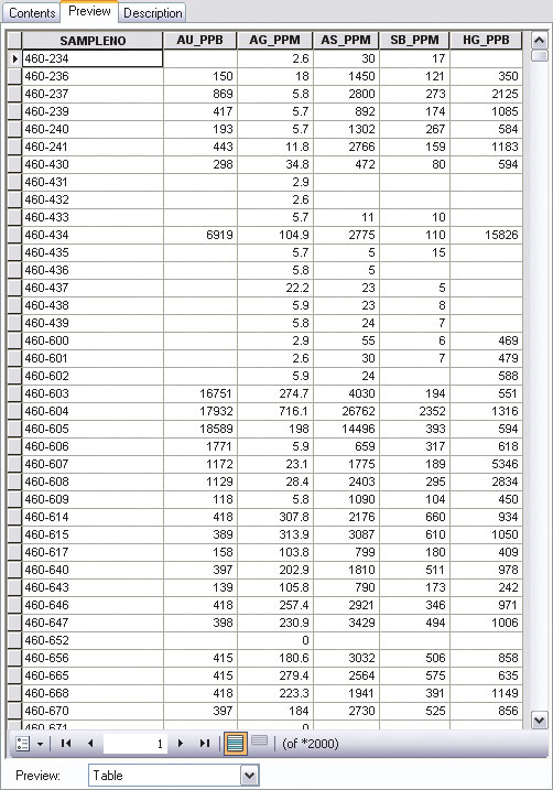
When CSV files are viewed in ArcCatalog, many records have blank fields.
Prepare a Composite Spreadsheet
HSSR_LonLat83.xlsx contains 96 sample sites collected as part of the HSSR back in the 1970s and 1980s. This data is often used as part of a regional reconnaissance program. Prepare the HSSR data for import.
- In Excel, open HSSR_LonLat83.xlsx. Save a copy to work with and name it HSSR_LonLat83_Import.xlsx. Inspect this data and fix any field headers that don't follow the rules. Make sure to check for spaces in field header names.
- The major fix will be to change the percent (%) symbol to the letters PCT. Use Replace by selecting the first row and pressing Ctrl + R to perform that task quickly.
- Create a named range called HSSR_Import_R and make sure it includes those header fields. Save this file.
Managing CSV Files in a Text Editor
Now to prepare the Rock and Soil analytic data for proper import—a much more difficult task. First, you will use a text editor to prepare Soil_Data.csv.
- Using Windows Explorer (or another file manager), navigate to \Battle_Mountain\XLSFiles and open Soil_Data.csv in WordPad. (Note: If CSV files are opened in Excel by default on your machine, right-click the file, choose Open With, and select WordPad.)
- Immediately save this file as Soil_Data_Import.csv.
- Notice that field names are properly constructed and that much of the analytic data is numeric. However, there are many records that contain < characters before a numeric value.
These records each contain less than the minimum detectable amount of a specific element. Sometimes, a sample contains more than a maximum detectable amount. These samples are usually coded with a greater than (>) symbol (e.g., >10,000 for gold). Fortunately, the over-limit samples in this dataset have already been resolved, so only the less than values need fixing.
Since it is statistically meaningful to recognize that some small amount of each element exists in all samples, it is not appropriate to change all < values to zero. Instead, change them to a smaller absolute value, typically 20 to 50 percent of the detection limit. Take a more conservative approach and use 20 percent. Table 1 lists the current value and smaller absolute value for elements below the minimum detection limit.
| Element | Abbr. | Unit | Detection Limit | Change From | Change To |
|---|---|---|---|---|---|
| Antimony | Sb | PPM | 5.0 ppm | <5 | 1 |
| Arsenic | As | PPM | 5.0 ppm | <5 | 1 |
| Gold | Au | PPB | 5.0 ppb | <5 | 1 |
| Mercury | Hg | PPB | 10.0 ppb | <10 | 2 |
| Silver | Ag | PPM | 0.5 ppm | <0.5 | 0.1 |
- In WordPad, move to the top of the document and begin by replacing the values for antimony. Select Replace (shortcut: press and hold the Ctrl and H keys) and (based on the values shown in Table 1) set Find to < 0.5 and Replace All to 0.1. Use Find and Replace All to change all values below the detection limit for arsenic, gold, mercury, and silver with the values shown in Table 1. When finished with the last element, perform one more Find for both < and > symbols to confirm that all the above and below limit values were found. You will see that the one sample below the minimum level for silver (Ag) was listed as <0.2 rather than <0.5. Change it to 0.1. Save and close the file.
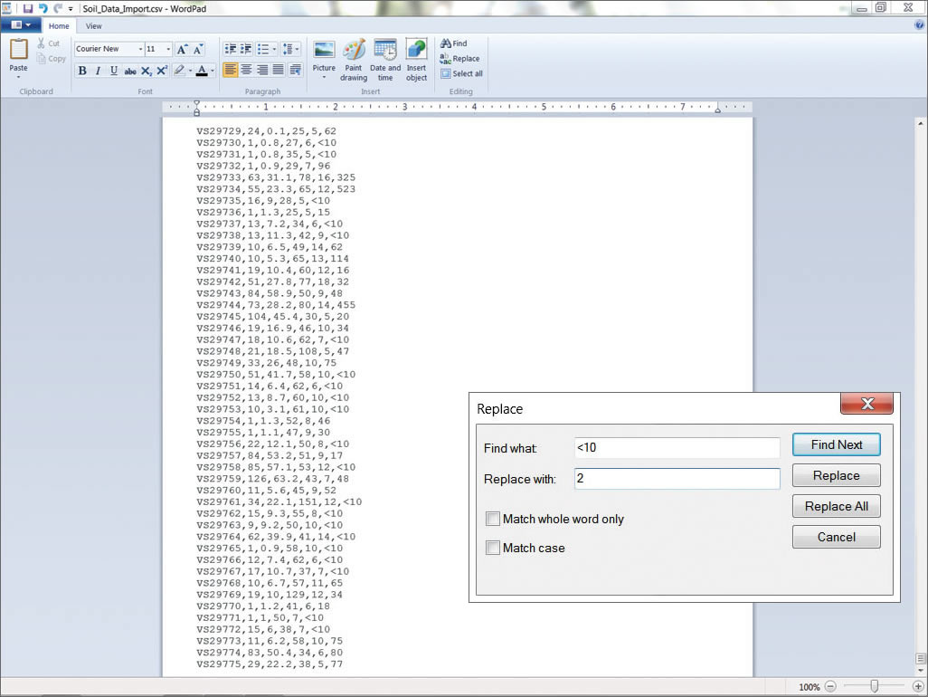
When the same file is viewed in WordPad, blank fields contain values preceded by a < or > symbol. These indicate values below the detection limits and will be replaced using values in Table 1.
Managing CSV Files in Excel
Now, try a similar approach with Rock_Data.csv, using Excel to replace undesirable values. This approach is much more powerful, but also dangerous.
The danger with using Excel to edit and format analytic data lies in how it uses leading zeros to manage alphanumeric strings when all other characters are numeric. Excel tends to convert leading zero strings to numeric values, which forever changes the data. This can be especially dangerous when working with datasets such as tax parcels and lab samples. However, if the file is saved from Excel back into a CSV file, the leading zeros are gone forever and there are no problems.
- In Windows Explorer, find Rock_Data.csv and open it in Excel. Immediately save the file as Rock_Data_Import.xls so you have the original CSV file and this copy in Excel.
- Inspect the file and look for improper field names and inappropriate data formats. Note that numeric data aligns on the right side of a cell, while alphanumeric data aligns on the left. Note that alphanumeric data that did not show up in most fields when previewed in ArcCatalog is now visible in Excel.
- Repeat the same Find and Replace All steps performed on Soil_Data_Import.csv in WordPad using the replacement values in Table 1. Note that the numeric values align on the right.
- Search for the < and &tt; characters to confirm that all the above and below limit values have been found. Another sample below the minimum level for silver (Ag) was listed as <0.2 rather than <0.5. Edit the cell manually to change the value to 0.1. Save the file.
- Next, manually format columns to reinforce numeric data formats. Select Column A by right-clicking its header, select Format Cells, and choose Text. Right-click columns B, D, E, and F and format as Number with no (0) decimal places. Right-click Column C and format as Number with one decimal place.
- Save the file as a CSV file, then reopen it in Excel and save it as an XLS file.
- In the last step in preparing the Rock_Data_Import.xls, create a named range containing all the cells and name it Rock_Data_Import. Now the data can be imported into an ArcGIS geodatabase. Save the file and close Excel.
Once all tables have been carefully prepared, they are imported into a new file geodatabase called Geochemistry.
Building the Geodatabase (Finally)
As the final step in this exercise, you will create a geochemistry geodatabase and import the Excel named ranges and CSV files.
- Open ArcCatalog and navigate to \Battle_Mountain\GDBFiles. Preview the Battle_Mountain.mxd file and review the layer files and the geodatabase layers in the Battle_Mountain file geodatabase.
- Right-click the Battle_Mountain\GDBFiles folder, select New > File Geodatabase, and name it Geochemistry.
- First, test a single table import of an Excel named range by right-clicking the new Geochemistry geodatabase and selecting Import > Table (single).
- In the Table to Table wizard, set Input Rows by browsing to \Battle_Mountain\XLSFiles and opening Sample_Location_Import.xls. In the Input Rows dialog box, select Rock_Locations_Import_R.xls, the named range created previously. Name the output table Rock_Locations_Import, accept all other defaults, and click OK. The rock sample locations are added as a geodatabase table.
- Open the table and verify that the import was successful. Pay special attention to field names and formats to make sure they were imported correctly. If not, check that you imported the correct file and that the named range included the field names. Make any corrections and reimport the file.
- Continue populating the geodatabase by adding the rest of the tables. Right-click the Geochemistry geodatabase and select Import > Table (multiple).
- In the Table to Geodatabase (multiple) wizard, load all remaining tables, including three tables created from Excel tables located in \Battle_Mountain\XLSFiles:
\Sample_Locations_Import.xls\Soil_Locations_Import_R
\HSSR_LonLat83.xls\HSSR_Import_R
\Rock_Data_Import.xlsx\Rock_Data_Import_R
and one CSV file:
\Soil_Data_Import.csv. - Click OK and watch as the four files are imported.
Because you carefully defined these import datasets, the ArcGIS data geoprocessing function readily uses the assigned names.
Finally, open each table in ArcCatalog and verify field names, formats, and record counts. You successfully outmaneuvered those tricky % characters. Finally, remove the _Import from each geodatabase table name and take a break.
Conclusion
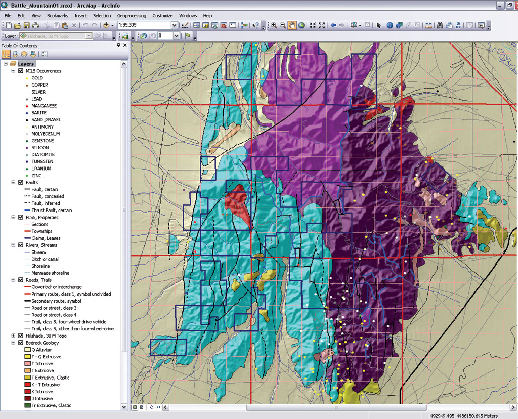
If you preview the Battle Mountain geologic map or open the Battle Mountain MXD, you will see the bedrock geology, geologic structure, and mineral occurrences in the study area. Wouldn't it be interesting to place all these rock, soil, and stream sediment samples in this model and go prospecting? This model is designed to do just that. The geochemical data can be used to analyze favorable ratios between multiple elements, define spatial relationships between rock units and faulting, and compare your data to current mines and past producers.
Acknowledgments
The data used in this exercise was originally developed as part of an ArcView GIS 3 mining training program. While the sample data is synthetic, it is true to the underlying geology. While landownership is imaginary, it reflects exploration trends around Battle Mountain, Nevada, in the early 1990s. Bedrock geology was derived from the Nevada Bureau of Mines and Geology County mapping series. HSSR data was developed through the US Department of Energy National Uranium Resource Evaluation (NURE) program. All data has been transformed from UTM North American Datum 1927 (NAD27) into the current NAD83 datum.