ArcUser
Fall 2012 Edition
Unlocking Data Trapped in Paper
Address geocoding legacy geological data
By Mike Price, Entrada/San Juan, Inc.
This article as a PDF.
What You Will Need
- ArcGIS 10 for Desktop (Basic, Standard, Advanced editions) with service pack 5
- An Internet connection
- The sample dataset
- An unzipping utility such as WinZIP
About the Sample Dataset
The exercise uses the same data from Battle Mountain, Nevada, that was used in two recent ArcUser tutorials. Both the tabular and polyline geophysical datasets are synthetic but match the area's underlying geology and work with the synthetic soil dataset previously used. It is similar to data packages that were developed prior to the early 1980s when the use of small computers for data development, mapping, and charting was beginning to evolve. Landownership is also fictitious. Bedrock geology was derived from the Nevada Bureau of Mines and Geology county mapping series. The Hydrogeochemical and Stream Sediment Reconnaissance (HSSR) data used was developed by the US Department of Energy National Uranium Resource Evaluation (NURE) program.Editor's note: In this tutorial, geologist and GIS modeling guru Mike Price shares a novel strategy for making old datasets trapped in non-spatially-aware formats available for use in GIS.
The exercise, set in Battle Mountain, Nevada, uses tabular and polyline geophysical datasets that are synthetic but match the area's underlying geology.
Every now and then, geologists encounter an impossibly old dataset that might be very useful in a modern exploration setting. There are several strategies for dealing with this situation. The data can be brought into a digital format by scanning, georeferencing, and digitizing paper maps and cross sections. Old printed tables can also be scanned and digitally recognized. In extreme cases, the data in printed tables can be entered—one record at a time—into a modern digital data format.
When I began my career as a field geophysicist in the early 1970s, most of my field data was hand entered into field books or stenographer's notepads. Field locations were often crudely sketched on topographic maps. If I was lucky, these records included a surveyed project baseline and a perpendicular reference of origin with beginning stations. The field crew was responsible for maintaining a true course along all survey lines and measuring the distance between stations. The times—and field procedures—have certainly changed.
This exercise takes up the challenge of making an impossibly old dataset and field map fit into the modern digital world. This exercise expands the Battle Mountain, Nevada, training model used in "Prospecting for Gold: Building, mapping, and charting point geochemical data," a tutorial that ran in the summer 2012 issue of ArcUser. Some legacy subsurface electrical methods geophysical data was added to the data on the soil geochemical anomaly identified in that exercise. This legacy data was obtained in the 1980s using traditional methods. Lines were surveyed using the compass and pace method. Fortunately, the field geologist had a new personal computer and a spreadsheet program. He used both to compile and model the field data. However, survey lines he used were supplied in a paper map.

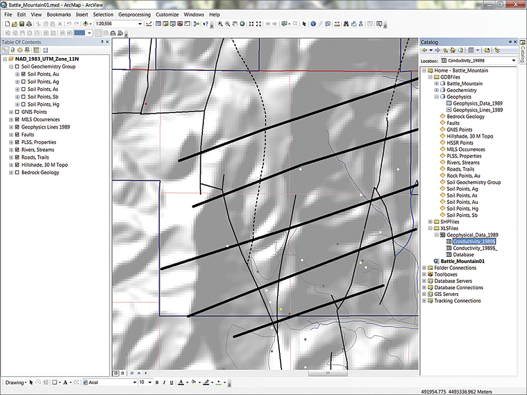
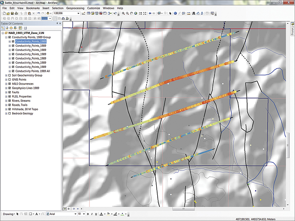
Use the Add Data tool to add the digitized traces of the survey lines to the map and symbolize them with a wide line.
Getting Started
To begin this project, download the sample dataset for this article. Verify that ArcGIS 10 for Desktop has service pack 5 applied.
Unzip the training set into a new folder, separate from any other training data used for previous exercises, and inspect the data. The root folder contains an ArcMap document called Battle_Mountain01 and three subfolders. The SHPFiles folder contains a polyline shapefile of the 1989 survey lines. The XLSFiles folder holds an Excel spreadsheet containing processed geophysical data listing the conductivity of rocks below the survey lines. Let's check out these two files and see how this data can be added to the map.
Exploring Battle Mountain
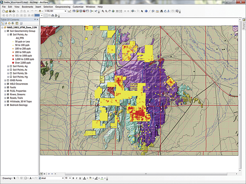
Start an ArcMap session and open Battle_Mountain01. Scan the map to familiarize yourself with the Battle Mountain area. The cluster of bright red points in the central area represents a significant precious metals anomaly, detected during a recent geochemical survey. Does something important lie underneath these points?
The cluster of bright red points in the central area represents a significant precious metals anomaly, detected during a recent geochemical survey.
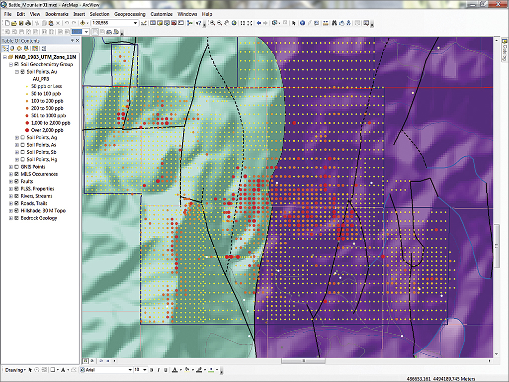
Choose Bookmarks > Anomalous Soil 1:20,000 to zoom to an area of the map. Explore this area carefully. Turn on the labels for the Bedrock Geology polygon layer and look at the bedrock units, including the Harmony, Valmy, and Pumpernickel Formations, and two larger lithologic groups, the Crane Canyon and Antler sequences. By using the Identify tool on the faults in these areas, you can see that the area of interest is crossed by many high angle normal faults and remnants of several horizontal thrust faults. Is it possible that these faults, cutting a variety of geologic units, could influence mineralization?
Fortunately we have information from an early geophysical survey that measured the area's resistance to electrical flow and have several digitized survey lines and files containing information about the conductivity (the opposite of resistivity) of the underlying rocks. Because metal-bearing rocks often contain significant pyrite, pyrrhotite, and other conductive sulfide minerals, a conductive precious metals ore body can sometimes be located and defined using this information. The first step is to map and analyze this conductivity data.
Add the Conductivity_1989$ worksheet for the Battle_Mountain\XLSFiles folder to the map.
Preparing to Post and Map Legacy Geophysical Data
The old paper map shows that five survey lines cross the prospect from southwest to northeast, generally perpendicular to regional faulting. These lines are stored in a shapefile, Geophysics_Lines_1989, located in the \SHPFiles\UTM83Z11\ folder. Use the Add Data tool to add the digitized traces of the survey lines to the map. Symbolize these survey lines with a wide line. Notice that the lines are not quite parallel, nor are they perfectly straight. Just how did they do this before GPS?
Mapping Survey Lines
Next, create a new geodatabase in the project folder and export the survey lines into it. Open the ArcCatalog window in ArcMap, navigate to the Battle_Mountain\GDB files\ folder, and create a new file geodatabase named Geophysics. Right-click the Geophysics geodatabase and choose Import. Navigate to SHPFiles\UTM83Z11\ and choose Geophysics_Lines_1989. Keep the same name for the feature class, add it to the map, and delete the original shapefile. You could also simply change the data source for the Geophysics_Lines_1989 layer from the original shapefile to the new feature class. Open the attribute table and review the attributes. Save the map.
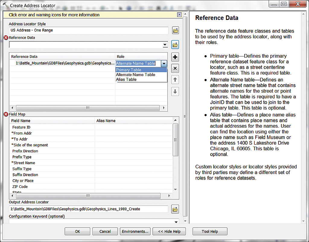
To create a new address locator, right-click Geophysics, select New > Address Locator, and specify the US Address—One Range style.
Exploring Legacy Point Data
Now to look at the tabular data in the XLSFiles folder. At least the data is in a spreadsheet, so it probably won't require much preparation. Add the Conductivity_1989$ worksheet from the Battle_Mountain\XLSFiles folder to the map.
Open the Conductivity_1989$ table and note that each record includes a line name ([Line_Name]) and a distance reference along the line ([Station_M]). Conductivity is measured in Siemens per meter. Each record includes the [N_Factor] (or depth below the surface defined by dipole geometry). However, there are no coordinates. How can these points be easily placed on the map or displayed in 3D?
I learned about geocoding early in my GIS career. At first, I imagined it was something special for geologists and was somewhat disappointed to learn that it was mostly used to place address strings as points on a map. However, shortly after this I needed to quickly map a table quite similar to this conductivity table. I imagined that if I could convert the line names and distances into something resembling street addresses, I might be able to geocode them. I tried it, and it worked. Let's try the same technique with the Battle Mountain data.
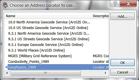
In the dialog box, click the Add button, navigate to the Geophysics geodatabase, and select the Geophysics_1989 address locator.
Preparing Geophysical Data for Geocoding
Inspect the [Line_Station] field and notice how geophysical points (stations) were often described on a survey line. Characters to the left of the plus (+) sign are the name of the survey line. The numeric characters to the right of the plus sign measure the distance along the line. Imagine the distance along the line as the address numeric and the line designator as the street name. If the order of these elements was reversed, these records should geocode using a numeric, range-based centerline geocoding method.
To work, this would just require adding and populating one new field. But wait, this is a Microsoft Excel spreadsheet that can't be edited inside ArcMap. This can be solved simply by exporting this Excel worksheet to the Geophysics geodatabase. Right-click the Geophysical_Data_1989$ table, choose Data > Export All Records to \Battle_Mountain\GDBFiles\Geophysics.gdb, and name it Conductivity_Table_1989. Open this table and verify the new table has 5,287 records and delete the Geophysical_Data_1989$ table from the map. Save the map.

After the first geocoding pass, more than 900 points were not geocoded.
Add a new 20-character text field named [Address2]. Right-click [Address2]. Open the Field Calculator by right-clicking a field header and use it to create this expression: [Station_M] & " "& [Line_Name]. Make sure String is selected for Type. Click OK. The calculated field should contain records for the contents of both the [Station_M] and [Line_Name] fields (e.g., 145 Line 250S). If the calculated data does not conform to this format, check the formula and recalculate the field.
Creating a One Range Address Locator
Now to build an address locator in ArcCatalog. Close ArcMap and open ArcCatalog.
- Open the Geophysics_Lines_1989 table and make sure all the fields necessary for a One Range locator are present. With a One Range locator, all address elements are contained within a single field. The technique substitutes information about the survey lines for traditional geocoding elements. [Line_Name] represents the street name, [Line_Start] provides the From Addr, and [Line_End] is the To Addr. Because the method will geocode on a centerline, [ID] is a filler for the required street side parameter. Close ArcCatalog.
- Inside ArcMap, open the ArcCatalog window and navigate to Battle_Mountain\GDBFiles\Geophysics. Right-click Geophysics, select New > Address Locator, and specify the US Address—One Range style. Select Geophysics\Geophysics_Lines_1989 as the Reference Data. If the Role field in the dialog box defaults to Alternate Name Table, click that field and change the Role field to Primary Table.
- Now set the Field Map as shown in Table 1. In the output field, navigate to the Geophysics geodatabase and save the address locator as Geophysics_1989. Click OK to create this new address locator.
| Field Name | Alias Name |
|---|---|
| From Addr | Line_Start |
| To Addr | Line_End |
| Side of segment | ID |
| Street Name | Line_Name |
Geocoding the Data
Now this data can be geocoded along the digitized survey lines. First, right-click in an unused area of a toolbar and load the Geoprocessing toolbar.
On the Geoprocessing toolbar, click the Geocode Addresses button. In the dialog box, click the Add button, navigate to the Geophysics geodatabase, select the Geophysics_1989 address locator, and click OK.
In the next dialog box, set Address Input Field to Address2 and save the results as Conductivity_Points_1989 in GDBFiles\Geophysics.
Export the geocoding results as a feature class in the Geophysics geodatabase. Add it back to the map, apply symbology using a layer file, and make seven copies of the layer.
Click OK to start geocoding.
When the first pass finishes, you will have points that were not geocoded. Set Show results to Unmatched Addresses and inspect the problem records. Notice that all unmatched points have a score of 79. With this database, a minimum match score of 75 is acceptable, so change the minimum matching score from 85 to 75.
Click the Rematch button. In the next dialog box, click the Geocoding Options button and lower the score to 75. Click OK to close Geocoding Options and click the Rematch Automatically button.
Close any warning messages and watch as the remaining 956 points match successfully. Close the Geocoding wizard and save the map.
Now save the geocoding results as a feature class. Right-click Conductivity_Points_1989 and choose Export > Data to save the results as a feature class in the Geophysics geodatabase.
Let ArcGIS add the new feature class to the map and remove the original geocoding result set from the TOC. Doing this clears the current geocoding session from the map document and releases several locks on those files. Save the map again.
However, if you needed to return later to update or enhance the geocoding session, you would not remove the geocoding results from the TOC but would use the Review/Rematch Addresses option on the Geocoding toolbar to make changes.
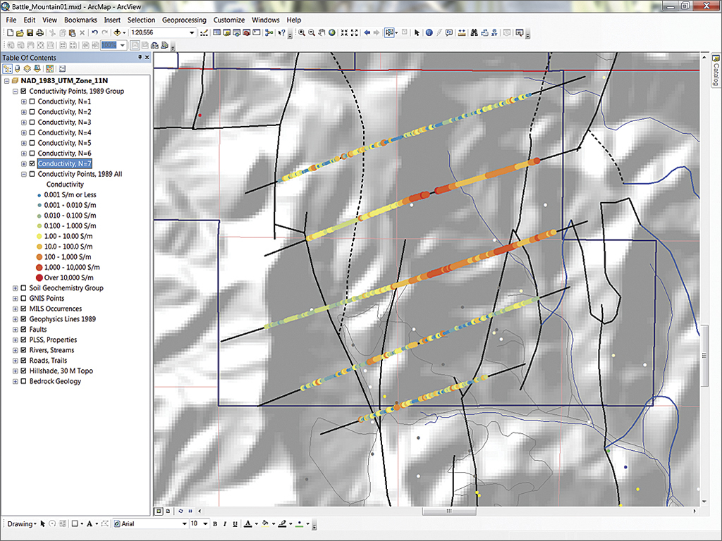
Use a definition query on each layer to split the points into separate layers by depth.
Symbolizing and Displaying Geophysical Data
Since conductivity for rocks may vary between 0.000001 and 10,000 Siemens per meter, I have created a simple logarithmic legend and stored it as a layer file. (For more information about rock resistivity/conductivity, check out the University of British Columbia website)
After adding the now geocoded conductivity points into the map, a predefined layer file can be used to assign symbology. The sample dataset contains layer files to expedite symbolizing the results. They are located in the GDBFiles folder. Double-click the Conductivity_Points_1989 layer in the TOC. Click the Symbology tab, then the Import button, and navigate to the Conductivity_1989 layer file and apply it.
Often warmer (red) colors and larger point sizes are used to show conductive (possibly mineralized) data. Use the Identify tool to check points on any line. Points are stacked as many as seven levels deep, coded by the integer [N_Factor] field. Higher N values represent deeper readings. Actual depths are defined by spacing of transmitter and receiver electrodes along each line.
Displaying Conductivity Data by Depth
Let's split the points into separate layers by depth and go gold prospecting (again).
To display points on separate levels defined by an N factor, first copy the Conductivity_Points_1989 layer seven times by right-clicking Conductivity_Points_1989 and choosing Copy. Next, right-click the NAD_1983_UTM_Zone_11N data frame and select Paste Layer.
Repeat the paste layer procedure six more times until you have eight instances of Conductivity_Points_1989.
Select all eight layers, right-click, and save them as a group layer called Conductivity Points, 1989 Group.
Start at the bottom of the group and rename that layer Conductivity Points, 1989 All.
Select the layer at the top of the group and rename it Conductivity N=1. To display only points at the N=1 depth by right-clicking on this layer, click the Definition Query tab and create the definition query "N_Factor" = 1.
Repeat the process to rename and create a definition query for the next six layers, using N=2, N=3, and so on. When finished, save the map.
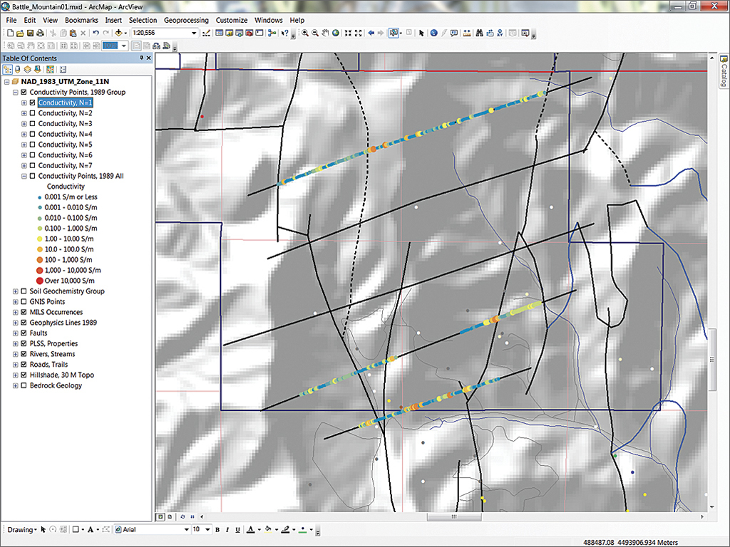
To display data level by level, from the surface down, turn off all Conductivity instances and turn on one instance at a time, beginning with N=1.
To display data level by level, from the surface down, turn off all Conductivity instances and turn on one instance at a time, beginning with N=1. What do you see?
In this simple model, big red points represent conductive rocks. Their conductivity is probably related to high sulfide content and could possibly indicate associated gold, silver, and copper mineralization. The previous exercise using Battle Mountain data mapped US Bureau of Mines Mineral Industry Location System (MILS) points and explored the multiple styles of mineralization in this area. Surface MILS points in the anomalous area show evidence of silver and lead, as well as instances of gold, antimony, and even copper. This could be the next Comstock Lode. Notice that shallow conductivity occurs primarily on Lines 250N and 750N. At depth (N=7), conductive rocks are much more pervasive. Perhaps we should look at this data a little more closely.
Digging Deeper
In this exercise, we successfully incorporated legacy geophysical data using a simple one-range address locator. The data was digitized survey lines and a spreadsheet with a spatial reference consisting only of line names and station distances along the lines. Using this simple methodology, 5,000 data points were posted to the map in just a few minutes.
Can this approach be used for data from other traditional sampling methods such as line-based soil geochemistry, surface trench samples, underground face samples, and underground longhole drilling? Why not? You just need to understand your data.