ArcWatch: GIS News, Views, and Insights
June 2012
Using Image Analysis Functions to Display Layer Tints on Hillshades
Using transparency to overlay colored rasters on hillshade or other grayscale rasters results in a washed-out, less detailed image. This tip will show you how to create an image that instead retains the original colors and details by using the No Alteration of Grayscale or Intensity (NAGI) fusion method. This method is extremely versatile, so it can be used whether you are working with mosaic datasets or image analysis functions in ArcGIS 10 for Desktop and above. It also works with color ramps and color map files.
The tip "Learn a New Method for Displaying Hillshades and Elevation Tints," published in the March issue of ArcWatch, explained how to use the NAGI fusion method with mosaic datasets and color map files. This tip explains how to fuse a grayscale and colored raster using color ramps and functions available through the Image Analysis window. A map of Washington state elevation was selected to illustrate how to use the NAGI fusion method.
Solving the problem described above—a washed-out image with less detail—often involves transparently overlaying a hypsometric tint on a hillshade. This is a common method for symbolizing terrain. A hypsometric tint is often displayed using a color ramp with colors that represent different elevations (figure 1).
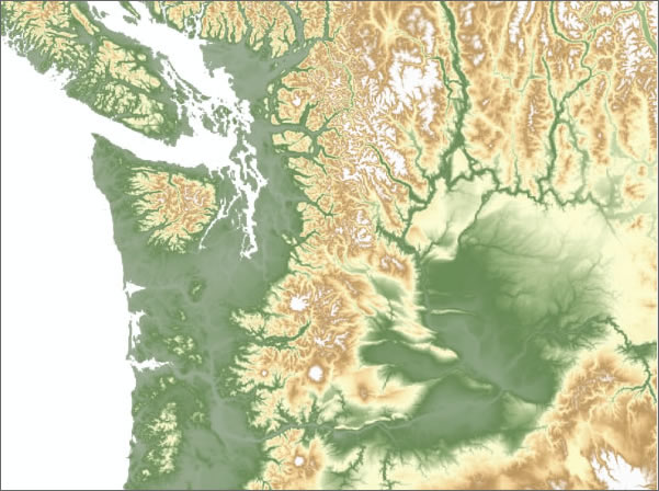
Figure 1. A hypsometric tint showing elevation
A hillshade of a digital elevation model (DEM) is often displayed as a grayscale raster (figure 2).
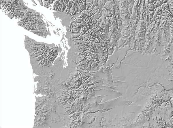
Figure 2. A grayscale hillshade
When the hypsometric tint is displayed transparently over the hillshade, the result is a washed-out version of the hypsometric tint and a less detailed version of the hillshade (figure 3).
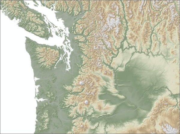
Figure 3. The result when the hypsometric tint is shown with 40 percent transparency over the hillshade
The NAGI fusion method produces a better result because the intensity of the original colors and the detail in the grayscale raster are retained (figure 4).
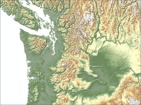
Figure 4. The result when image functions are used to control the display
At the core of this display method is a combination of pan sharpening, contrast stretching, and gamma stretching functions. The pan sharpening function uses a panchromatic and multispectral, three-band RGB (red, green, blue) raster as input. In this tip, the inputs are a hillshade created from a DEM as the panchromatic raster and a DEM with a color ramp that has been converted to a multispectral raster. The output from the pan sharpening function is then used as input for the contrast and gamma stretching functions.
Step 1. Since layer-tinted DEMs are not usually managed as three-band RGB rasters, a conversion is required. To do this, add the DEM to ArcMap, right-click the layer in the table of contents, and click Properties. On the Symbology tab, select the color ramp you want to use to display the data. Click OK to close the Layer Properties dialog box. Right-click the layer in the table of contents, click Data, and click Export Data. In the Export Raster Data dialog box, check Use Renderer and check Force RGB. Choose a location and file name, then click Save. Choose to add the exported data to the map as a layer. The three-band RGB image will be added to the table of contents.
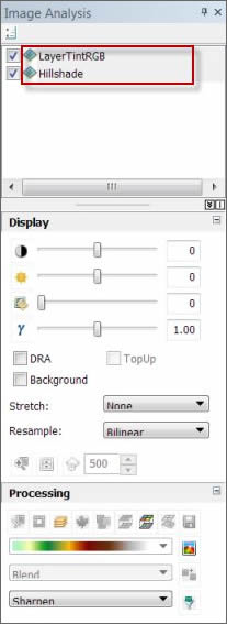
Figure 5. The Image Analysis window
At this point, you can either use the method described in the earlier tip to add the raster to a mosaic dataset and render it, or you can follow the instructions below to use the Image Analysis tools.
Step 2. Next, set up the layer tint and hillshade rasters to use the pan sharpening function. Add the grayscale hillshade and multispectral RGB layer tint rasters to ArcMap, if they have not already been added. In standard tool bar, choose Windows > Image Analysis. In the top section of the Image Analysis window, select both the hillshade and RGB rasters using the Ctrl key to click each raster's name to highlight it (figure 5, at right).
Step 3. Now you can use the pan sharpening function. Click the Pan Sharpening tool in the Processing section of the Image Analysis window. This will create a new layer, which will be positioned as the top layer in the Image Analysis window. In the Image Analysis window, right-click the newly generated pan sharpening layer and click Properties. On the Functions tab, right-click Pansharpening Function and click Properties. On the General tab of the Raster Function Properties dialog box, change the Output Pixel Type to 8 Bit Unsigned; this data type is required so that you can use the pan sharpening function in the next step.
Step 4. Modify one of the options in the pan sharpening function. On the Pan Sharpen tab, change the Method parameter to Simple Mean. Retain the rest of the defaults and click OK.
Step 5. Next, apply a contrast stretch and a gamma stretch. Right-click Pansharpening Function, click Insert, and click Stretch Function to apply a contrast stretch. Change the Type to Minimum-Maximum. Check the Use Gamma option. In the Gamma section of the dialog box, check the Use Gamma option and change the Gamma value from 1.0 to 0.5 for each of the three bands. In the Statistics section of the dialog box, type "5" as the Min value and "215" as the Max value for each of the three bands. The final function chain will look like figure 6.
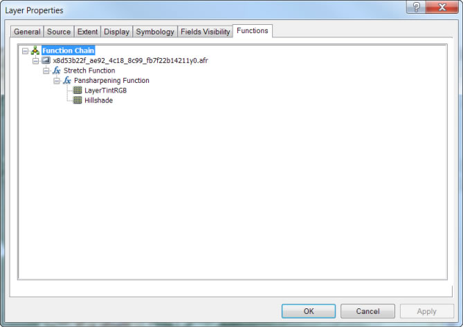
Figure 6. The final function chain
Click OK to check your results.
After checking the results, feel free to experiment by resetting the gamma function or changing the minimum and maximum values for in the Stretch Function.
Step 6. Creating this display using the Image Analysis window instead of mosaic datasets will produce a temporary raster. If you want to keep your results, export the layer from ArcMap. To do this, right-click the layer in the table of contents and click Export Data.
The data you save can now be added to an ArcMap session, and it will be displayed with the final results.
If you want to try this out yourself, download this .zip file, which contains a map package of the Washington state elevation map used in this article.