ArcUser

Fall 2012 Edition

Empirical Bayesian Kriging

Implemented in ArcGIS Geostatistical Analyst

By Konstantin Krivoruchko, Senior Research Associate, Software Development Team, Esri

This article as a PDF.

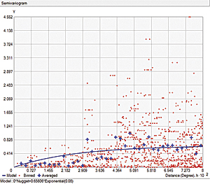
Figure 1a: The semivariogram values for the pairs of points (red), their averages (blue crosses), and the estimated semivariogram model (blue line.)

Obtaining reliable environmental measurements can be costly and laborious, and in many cases, environmental contaminant samples are not collected where people live or work. The ability to predict values where observations are not available is, therefore, very important. Interpolation is the process of obtaining a value for a variable of interest at a location where data has not been observed, using data from locations where data has been collected.

There are many methods for interpolating spatial data. They fall into two broad classes: deterministic and probabilistic. Deterministic methods use predefined functions of the distance between observation locations and the location for which interpolation is required (for example, inverse distance interpolation). Probabilistic methods have a foundation in statistical theory. These predictors quantify the uncertainty associated with the interpolated values. The requirement of providing information on prediction uncertainty limits the choice of interpolators to statistical ones.

Development of reliable automatic statistical interpolation models has been a hot issue in the GIS community for a long time. However, this is a very challenging task because each statistical model is based on the users' data and the data is often so complex that it is extremely difficult to describe it mathematically without interaction.

Figure 1b: The spectrum of the semivariogram models produced by EBK

This article briefly discusses statistical interpolation features and then provides some details about the empirical Bayesian kriging (EBK) model implemented in ArcGIS 10.1 Geostatistical Analyst. Extensive testing using a large variety of data showed that EBK is a reliable automatic interpolator. This kriging model is also available as a geoprocessing tool that can be used in ModelBuilder and Python scripts.

Kriging

Kriging is the name given to a class of statistical techniques for optimal spatial prediction. It was developed by Lev Gandin in 1959 for meteorological applications. It has been used in many other disciplines, including agriculture, mining, and the environmental sciences.

Kriging is a probabilistic predictor and, as such, assumes a statistical model for the data. Kriging predictors have standard errors that quantify the uncertainty associated with the predicted values. Kriging predictors are called optimal predictors because the prediction error is minimized and, on average, the predicted value and the true value coincide. Kriging predictors:

Have smaller prediction uncertainty than other prediction models
Have the ability to filter out measurement errors
Use information on the correlation between the variable of interest and covariates

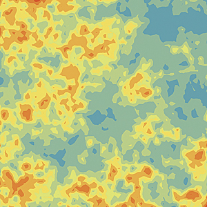
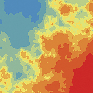
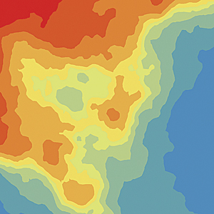
Figure 2: Spatial data simulated using power semivariogram model with power values of 0.1, 1.0, and 1.9 (from top to bottom)

When kriging predictors are applied to the analysis of radioactive contamination, they can answer questions such as, What is the probability that food contamination exceeds the radioecological standard at the specified location? and provide estimates of average and total contamination in specified areas.

Kriging uses a semivariogram—a function of the distance and direction separating two locations—to quantify the spatial dependence in the data. A semivariogram is constructed by calculating half the average squared difference of the values of all the pairs of measurements at locations separated by a given distance h. The semivariogram is plotted on the y axis against the separation distance h.

Figure 1a shows the semivariogram values for the pairs of points (shown in red) and their averages for a set of the distance intervals between the points (shown as blue crosses). The blue line in Figure 1a shows the estimated semivariogram model. This semivariogram model is then used to define the weights that determine the contribution of each observed data point to the prediction of new values at unsampled locations.

There are some statistical assumptions behind kriging. The main assumption is stationarity (spatial homogeneity). If data is stationary, the data mean and the semivariogram are the same at all locations in the data extent. If this assumption is held, just a few kriging model parameters have to be estimated from the data to make optimal predictions and valid statistical inferences.

If the data distribution is Gaussian, the best predictor is one that uses a linear combination of the nearby data values. For other distributions, however, the best predictor is often nonlinear and, therefore, more complex. The data can be transformed to follow a Gaussian distribution. Then it is possible to accurately back transform kriging predictions to the original data scale, which can be done in ArcGIS Geostatistical Analyst.

Classical kriging also assumes that the estimated semivariogram is the true semivariogram of the observed data. This means the data was generated from Gaussian distribution with the correlation structure defined by the estimated semivariogram. This is a very strong assumption, and it rarely holds true in practice. Hence, action should be taken to make the statistical model more realistic.

Introducing Empirical Bayesian Kriging

EBK differs from classical kriging methods by accounting for the error introduced by estimating the semivariogram model. This is done by estimating, and then using, many semivariogram models rather than a single semivariogram. This process entails the following steps:

A semivariogram model is estimated from the data.
Using this semivariogram, a new value is simulated at each of the input data locations.
A new semivariogram model is estimated from the simulated data. A weight for this semivariogram is then calculated using Bayes' rule, which shows how likely the observed data can be generated from the semivariogram.

Figure 3a: Predictions of the radiocesium soil contamination in six data subsets

Steps 2 and 3 are repeated. With each repetition, the semivariogram estimated in step 1 is used to simulate a new set of values at the input locations. The simulated data is used to estimate a new semivariogram model and its weight. Predictions and prediction standard errors are then produced at the unsampled locations using these weights.

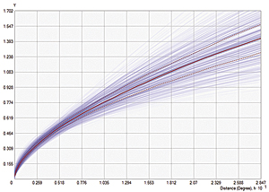
This process creates a spectrum of semivariograms. Each semivariogram is an estimate of the true semivariogram from which the observed process could be generated. Figure 1b shows the spectrum of semivariogram models plotted together. The median of the distribution is shown with a solid red line. The 25th and 75th percentiles are colored with red dashed lines. The width of the blue lines is proportional to the semivariogram weights so that the models with smaller weights are shown by thinner lines.

The default kriging model in EBK is called the intrinsic random function of order 0, and the spatial correlation model is the power model where b, c, and α (the allowed value of the power value α is between 0 and 2) are the model parameters. This correlation model corresponds to fractional Brownian motion, also known as the random walk process. It consists of steps in a random direction and filters out a moderate trend in the data.

Figure 3b: Fruit Basket by Giuseppe Arcimboldo (ca. 1527–1593)

Figure 2 shows simulated surfaces with three different power values of α: α=0.1 (top), α=1 (middle), and α=1.9 (bottom). Zooming in on any part of the surface shows a similar random walk surface. The correlation model with α=1, a linear model shown in the middle image, corresponds to the regular Brownian motion, process with independent step increments. However, the increments are dependent on fractional Brownian motion. If there is an increasing pattern in the previous steps, then it is likely that the current step will increase when the power value of α is greater than 1 and decrease when α is less than 1. In Figure 2, the simulated surface with small α (top image) looks like a mixture of a moderate trend and random noise while the simulated surface with large α (bottom image) shows nearly noiseless large scale data variation.

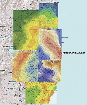
To demonstrate the use of EBK, six data subsets of measured radiocesium (¹³⁷Cs) soil contamination were modeled for locations near the Fukushima Daiichi Nuclear Power Station in Japan following the accident that occurred at that facility in 2011. They are shown in Figure 3a. Maps of the results of each subset are qualitatively similar: they show the same characteristics as the maps in Figure 2. This demonstrates that the default EBK model provides a good method for predicting radioactive contamination for small areas.

Using a distribution of semivariogram models—instead of just one model—offers a big advantage over classical kriging models. However, EBK has several additional advantages: the model can be used to interpolate nonstationary data for large areas and the data can be transformed locally to a Gaussian distribution.

Figure 4a: The distribution of radiocesium soil contamination data in six data subsets

With the EBK model, in the case of large datasets, the input data is first divided into subsets of a specified size that may or may not overlap. In each subset, distributions of the semivariograms are produced. Then, for each location, a prediction is generated using a semivariogram distribution from one or more subsets. Each data subset uses models defined by nearby values, rather than being influenced by very distant factors, yet when all the models are combined, they create a complete picture, just like the "face" in the Giuseppe Arcimboldo painting entitled Fruit Basket is created by combining groupings of fruits (Figure 3b).

Although the default EBK model makes the data distribution of the residuals closer to a Gaussian distribution by removing the local trend, the residuals distribution can still be non-Gaussian. In this case, a model with the data transformation option may produce better predictions. In Geostatistical Analyst, this can be identified using the model diagnostics.

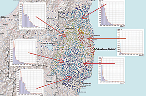
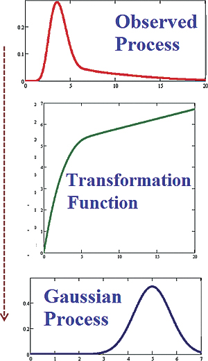
Figure 4b: The data transformation process

Plotting the ¹³⁷Cs soil contamination distributions in several areas of the data extent shows that they are clearly non-Gaussian and differ by region as shown in Figure 4a. Therefore, varying local data distribution clearly forms an essential feature of the optimal interpolation model. EBK provides an option to transform the observed process to a Gaussian process, using the estimated data transformation function as illustrated in Figure 4b.

EBK with the data transformation option estimates the data distribution many times using the following algorithm:

The data is transformed to a Gaussian distribution and a semivariogram model is simultaneously estimated from the data.
Using this semivariogram, new data is unconditionally simulated and then back transformed at each of the input data locations.
The new data is transformed and a new semivariogram model is simultaneously estimated from the simulated data.
Steps 2 and 3 are repeated a specified number of times. Each repetition produces a new transformation and semivariogram.
Weights for the semivariograms are calculated using Bayes' rule.
Predictions and prediction standard errors are made using weights and then back transformed with bias correction.

These associated prediction uncertainties should be considered when using these results for decision-making purposes. Figure 5a shows ¹³⁷Cs soil contamination prediction (Ci/km²) and prediction standard error maps produced by EBK for areas near the Fukushima Daiichi Nuclear Power Station. [A curie (Ci) is a unit used to measure the intensity of radioactivity of a sample.] Figure 5b shows the estimated ¹³⁷Cs distributions (with the median shown in red) for one location inside the data extent.

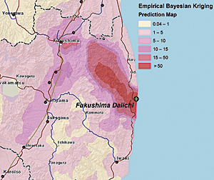
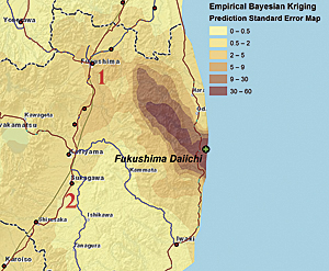
Figure 5a: ¹³⁷Cs soil contamination prediction and prediction standard error maps; 95 percent prediction intervals for locations labeled 1 and 2 are [7.82, 21.62] and [1.17, 3.21] Ci/km2.

Radioactive decay provides an interesting example because it is a Poisson process rather than the more straightforward Gaussian process. The essential property of any Poisson process is that its mean is equal to its variance. Therefore, the variability of the predictions tends to be smaller for observed data of lower values and larger for observed data with higher values. This is illustrated in Figure 5a.

Interpreting predictions together with the prediction standard errors provides a better understanding of possible contamination levels. Analyzing two labeled locations in Figure 5a in more detail reveals that the predictions and their associated prediction standard errors are (1) 14.72 and 3.52 and (2) 2.19 and 0.52.

The radioactive soil contamination at these locations is approximately (95 percent prediction intervals) 14.72 ± 3.52 × 1.96 ≈ 14.72 ± 6.9 Ci/km² and 2.19 ± 0.52 × 1.96 ≈ 2.19 ± 1.02 Ci/km², respectively. Therefore, the "true" contamination in the first location could be larger than 20 Ci/km², although the predicted value is smaller than 15 Ci/km². If the upper permissible limit of soil contamination is 15 Ci/km² (as it was in the former Soviet Union), living in the first location is rather unsafe and people living nearby should be evacuated. At the second location, the "true" contamination could be as much as 3 Ci/km², given a predicted value close to 2 Ci/km².

Conclusion

Empirical Bayesian kriging as implemented in the ArcGIS 10.1 Geostatistical Analyst extension provides both a straightforward and robust method of data interpolation. For more information on using EBK, see the online help for the ArcGIS Geostatistical Analyst extension. To learn more about spatial statistics, read Spatial Statistical Data Analysis for GIS Users published by Esri Press.

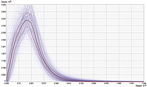
Figure 5b: Estimated ¹³⁷Cs soil contamination distributions at one location close to the Fukushima Daiichi Nuclear Power Station.

About the Author

Konstantin Krivoruchko is a senior research associate on the Esri software development team who played a central role in developing the ArcGIS Geostatistical Analyst extension. Prior to joining Esri in 1998, he was director of the GIS laboratory at the Sakharov Institute of Radioecology in Minsk, Belarus, where he developed GIS and spatial statistics curricula and supervised doctoral and graduate school candidate research pertaining to GIS applications and spatial statistical data analysis. He has taught numerous courses on applied spatial statistics and GIS. These activities are summarized in Spatial Statistical Data Analysis for GIS Users.

News