Turning a terabyte (TB) of lidar data into ready-to-use GIS products can be quite challenging. In this article, I share the strategies I used to transform lidar data into GIS products to benefit Washoe County, Nevada.
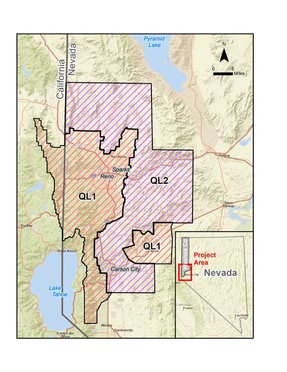
In 2017, the United States Geological Survey (USGS) 3D Elevation Program (3DEP), in cooperation with the Nevada Bureau of Mines and Geology (NBMG) and local cooperators, flew a lidar mission to collect quality level 1 (QL1) and quality level 2 (QL2) LAS data across more than 1,500 square miles covering Reno, Sparks, Carson City, and surrounding areas in northern Nevada. Local cooperators included the Washoe County Regional Basemap Committee (Washoe County, City of Reno, City of Sparks, and NV Energy), US Forest Service, Lyon County, and Storey County.
Deliverables for this project included classified LAS files, hydro-flattening break lines, digital elevation models (DEMs), digital surface models (DSMs), and intensity rasters. This project marked the first time the region has had such extensive lidar coverage, and the data received came with much promise as well as a number of challenges.
Moving Mountains of Data
In July 2018, the data—2,025 QL1 and 2,478 QL2 LAS files totaling 27.9 billion points—was delivered to Washoe County’s GIS program via a 1 TB external USB drive. It took a few weeks for network staff to make enough space available on Washoe County servers. At every step along the way, finding additional space for temporary files and managing intermediate products was a challenge. More than once, a batch process failed when it ran out of disk space.
One of the functions of Washoe County GIS is to respond to data requests. When engineering companies learned about the new lidar data, the county began getting requests for copies of the LAS files.
The lidar data was organized arbitrarily into 1,000-meter by 1,000-meter tiles that did not match the county’s township, range, and section (TRS) boundaries. Since TRS boundaries are typically used to locate an area of interest (AOI) for routine data requests, staff had to determine the specific LAS files that intersected the AOI a customer had requested and then copy those specific files.
To reduce this overhead, the county encouraged customers who were likely to make multiple data requests to bring in an external USB drive and get a copy of the entire dataset. A spare PC was dedicated to the hours-long copy operations so they wouldn’t interfere with other work. However, there is a certain level of risk when connecting external hardware into any network. Organizations with prohibitions against this would need other solutions for making the data publicly accessible.
Creating Derivative Products
While many engineering firms are quite happy to deal with LAS point clouds (and may even prefer them over contour lines), plenty of users still need traditional contours. Producing contours from lidar data is nothing new, but there are a few steps in the process that can trip the unwary.
Typically, lidar-derived contours appear noisy or jagged, which some users find objectionable. Instead of creating contours directly from the LAS dataset, it’s better to create them from a lidar-derived DEM. This introduces thinning and averaging into the process, resulting in better looking contours. (See ArcGIS help topic “Minimizing noise from lidar for contouring and slope analysis” for more information.)
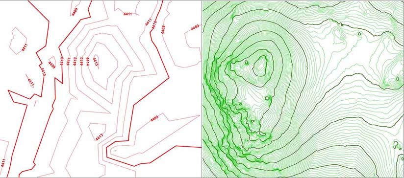
Contours created from lidar tend to have an excessive number of vertices, which can lead to large shapefiles. Decisions in the data processing chain must balance accuracy preservation against the practical considerations of data storage and distribution. DEM tiles could have been created from the LAS data, which would have allowed smoothing and thinning to be controlled to create a smoother DEM and more generalized contours with fewer vertices. However, by using the DEM tiles from the vendor, data manipulation was kept to a minimum and the output stayed true to the source data.
Repeat after Me, “Iteration Is Your Friend”
The amount of lidar data precluded processing the dataset all at once. Instead, a separate feature class of one-foot contours was produced for each of the more than 1,500 TRS sections covered by the lidar data. Significant portions of the lidar footprint extended beyond Washoe County’s boundary and fell outside the section grid typically used. The Bureau of Land Management (BLM) cadastral reference grid (Public Land Survey System [PLSS] First Division) was used to build a polygon layer covering the entire project footprint.
Irregular BLM section boundaries left gaps between some sections. Nevada’s “wide open spaces” have resulted in some strange PLSS boundaries. Editing the section boundaries ensured that all areas in the project had complete contour coverage. To create a single, seamless DEM from which to create contours, a mosaic dataset was built that referenced the DEM rasters for the QL1 and QL2 areas. Both QL1 and QL2 support a one-foot-interval contour.
A model, built using ModelBuilder in ArcGIS Pro 2.3, iterated through all section tiles and produced contours for each one. One big gotcha in this process: a single snap raster [which is used to align the cells of the output raster. Snap raster is set in the model’s Environment Settings] must be used for all the contouring operations. If this isn’t done, small differences in contour polyline outputs will result in edgematching errors between sections.
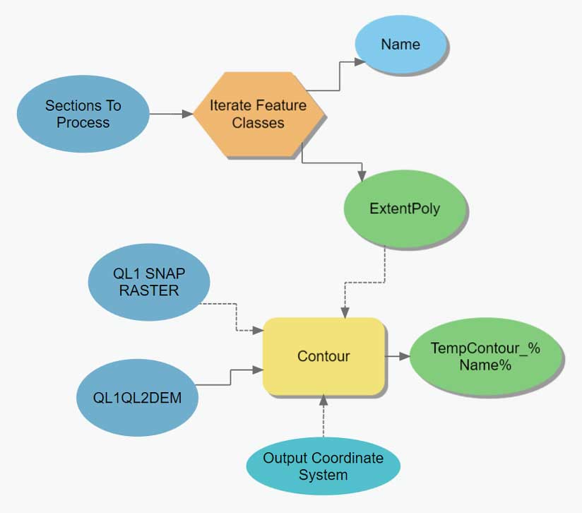
During the contouring operation, the output was reprojected into the State Plane Coordinate System used by Washoe County GIS. A z-factor of 3.2808 was applied to convert elevation from meters to feet. Because the contour operation created polylines within the minimum bounding box of the processing extent polygon, each contour feature class was clipped to the exact boundary of each section polygon to prevent overlaps in polylines between adjacent sections. Additional postprocessing included classifying the contours as either Index or Intermediate and exporting the finished contours to shapefile format for easy distribution.
Referenced Mosaic Datasets and Elevation Profiles
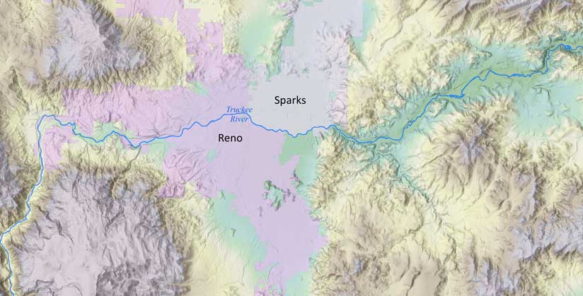
After creating a referenced mosaic dataset from the QL1-QL2 DEM, a multidirectional hillshade function was used to create a highly detailed hillshade for the entire project area. When set to 30 percent transparency and displayed over an elevation raster of the same DEM, this mosaic will improve Washoe County’s cartographic products.
Elevation profile charts are also easily derived from the DEM. By interpolating popular hiking trails to a 3D line using the DEM as an elevation source, a profile chart of the elevation gain along the trail can be created. This information can easily be made available to the public to help them make appropriate choices based on the level of hiking challenge desired.
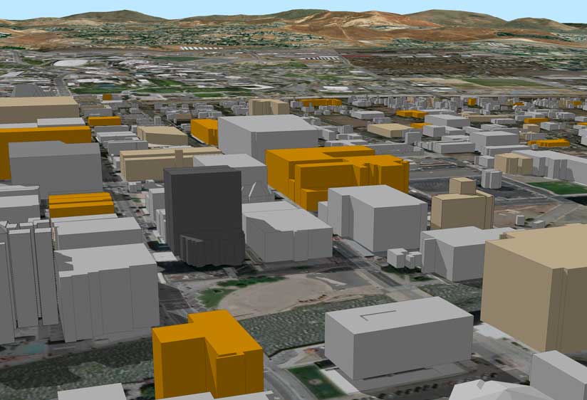
Roof Lines and 3D Buildings
Washoe County GIS traditionally maintains building footprints by heads-up digitizing from orthophotos. Lidar now provides an opportunity to not only update building footprints but also venture into the world of 3D buildings by creating 3D buildings for an area of suburban development where construction of new homes was in progress and for downtown Reno. There were no preexisting building footprints. The multipatch buildings were derived completely from lidar. The initial results are promising.
Science as Art
As a final example of the uses of lidar data in ArcGIS Pro, a 3D point cloud scene of downtown Reno was created. The lidar points were symbolized by elevation and modulated by intensity. Elevation shifts were symbolized from blue to green as elevation increased. Adding the modulation brings out contrasts in surface materials by increasing the brightness of high-intensity returns and reducing the brightness of low-intensity returns. This technique lends the scene an almost photographic quality. This high-tech art was professionally mounted and framed and now decorates Washoe County’s IT conference room.
Some Final Thoughts
There is plenty of value still to be extracted from the lidar data. Some of the potential tasks include merging the contours into a seamless dataset and creating simplified versions for use in web applications. I’ve barely scratched the surface of 3D visualization. Once I’ve finished generating the basic multipatch buildings, I look forward to adding textures to create more realistic 3D scenes.
Washoe County’s experience as a cooperator in the 3DEP program has been very positive and allowed the county input to the final coverage area, a chance to review the pilot project deliverables, and quick access to the final data—all for a relatively modest financial contribution. If your community has the opportunity to participate in a 3DEP project, I heartily recommend taking it.
For more information, contact Jay Johnson, of Washoe County GIS.
About the author