The United States is the world’s #1 net exporter of food. The American farmer, only 2% of the population, is unmatched in efficiency and productivity. The US Department of Agriculture (USDA) has been a scientific partner to American agriculture for over a century.
One of the products USDA produces in support of American agriculture is the USDA NASS CropScape cropland layer of the United States. CropScape helps gather statistics of cultivated land cover by tracking what crops are planted during a growing season, and where.
For the first time, CropScape has been published as a time series in the Living Atlas of the World, under the service name USA Cropland. Esri obtained NASS CropScape cropland imagery back to 2008, the first year all 48 conterminous US states were produced in one piece under the CropScape name. Esri assembled all eleven CropScape growing seasons since 2008 into a one-year-per-frame series that is ready for both analysis and animated display.
The Corn Belt
Or is it the Soybean Belt? Here in Le Mars, Iowa, we see the rotation between corn (yellow) and soybeans (green). By rotating soy and corn, farmers see higher yield in both products than in their respective monocultures. Soybeans are legumes which host nitrogen-fixing bacteria in their roots. These bacteria help take care of most of the plant’s nitrogen needs. As a result, soybeans can be part of a strategy which reduces fertilizer costs, increases yield for alternate year crops, and produces protein for feed. Soybeans yield a seed that is 40% protein, a valuable resource for feed and food processing.
The Ogallala Aquifer
In the semi-arid Oklahoma Panhandle we see circles, 1/4 mile across, where center-pivot irrigation is active. In a center pivot irrigation system, sprinklers or drippers move around in a circle, typically every three days. These farms are taking advantage of the Ogallala Aquifer, a large underground water resource that formed mostly between 2-6 million years ago, to grow wheat, corn, sorghum (milo), and other crops.

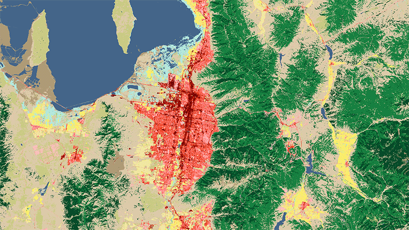
Rice in California
In parts of Northern California, there is water surplus in spring. During these times, the flat, clay soils of the Sacramento Valley tend to hold water like a big bathtub. Closest to the Sacramento River, natural levees form soils that are well drained, allowing for many crop choices. In recent years the crops in this area have been corn, tomatoes, sunflower, olives, almonds, and walnuts, among others. But away from the river, where soils are not so well drained, crop choices are restricted. A natural pairing for these kind of clay soils is rice agriculture. In this image you can see annual crops change in soils that are well-drained, while the dense-soil areas that grow rice (in periwinkle blue) grow it every season.

Try it!
Try this web map application which displays USA Cropland and USA NLCD Land Cover together in a time series, with multidirectional relief. Pause the time slider and click croplands in the map to see what crops were grown in any growing season from 2008 to 2018.
National Land Cover Dataset is masked out of the USA Cropland service by default
CropScape indicates what crop or crops were grown on cultivated lands in the USA during a growing season. But what about the non-cultivated lands? CropScape fills in these areas with land cover from NLCD, the National Land Cover Dataset. This is helpful because some agricultural lands (such as grazed and forested lands) are not tracked by CropScape. However, the NLCD data in non-cultivated areas changes only about every 5 years while CropScape cultivated lands change every year. As a result, some areas appear to change often while others do not. A lack of change could be due to a difference in data frequency, not from lack of change in the landscape.
Furthermore, in the time period after the 2018 CropScape was released in early 2019, the MRLC released a new set of NLCD datasets, going back to the year 2000, with 2016 as the most recent. As a result, the 2011 NLCD parts of the 2018 CropScape data were already out of date just a few weeks after the CropScape data was released in 2019.
For these reasons, Esri’s USA Cropland service has a bit different default behavior than what might be expected. The default processing template for USA Cropland, the analytic renderer, masks out non-cultivated areas. This helps make change analysis more accurate, since only what changes every year is enabled in the template. To display NLCD parts of the dataset that are turned off by default, you may instead choose the cartographic renderer in the set of processing templates.
But here’s a better suggestion. In your map, display the new time-enabled USA NLCD Land Cover service from the Living Atlas of the World directly beneath the USA Cropland service. We created a web map that gets this layer mashup started for you, that way you can make a copy and modify this map within the ArcGIS platform. There is also a web map application of this map that is pre-configured and ready to share.
Processing Templates Simplify Display
To display stock USDA colors with this service, or to help display a smaller, more targeted set of symbols, processing templates are available which display the top 10 products in US agriculture. These are Corn, Cotton, Rice, Wheat, Soybeans, Sugar, Oil crops, Fruit, Vegetables, and Nuts.


Commenting is not enabled for this article.