ArcGIS has supported hyperspectral data since the release of ArcGIS Pro 3.5. The earlier blog, Map Oaks, demonstrated the initial capabilities for analyzing AVIRIS hyperspectral imagery by collecting target spectral signatures directly from the imagery. Since then, hyperspectral analysis capabilities have continued to expand in ArcGIS Pro 3.6 and ArcGIS Pro 3.7, including support for USGS spectral library, a guided workflow through the Target Detection wizard, and additional detection algorithms.
With ArcGIS Pro 3.8 release, hyperspectral analysis has been further enhanced to support more hyperspectral imagery like AVIRIS-3 and AVIRIS-5 and provide new ways to create and work with spectral libraries. In addition to using spectral signatures from the USGS spectral library or collecting signatures directly from imagery, you can import in-situ spectral data stored in CSV files, such as the GLORIA dataset and HABs dataset, or extract spectral signatures from imagery using field geolocation data. These capabilities make it easier to incorporate field data into spectral-based hyperspectral image analysis.
Furthermore, the latest ArcGIS Online imagery updates bring hyperspectral analysis capabilities to the web. You can easily upload and share spectral library files (*.esl) using the new Esri Spectral Library item type and perform analysis using the three new web tools: Detect Target Using Spectra, Detect Image Anomalies, and Resample Library Spectra.
Now, let’s revisit the oak mapping workflow at the Jack and Laura Dangermond Preserve to demonstrate how field data can be used for spectral analysis in ArcGIS Online.
Step 1: Create a hyperspectral tiled imagery layer.
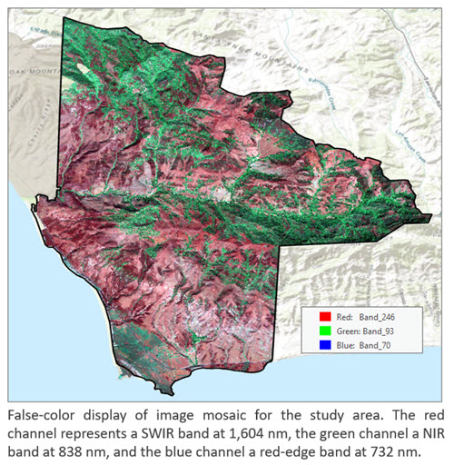
The hyperspectral imagery used in this study consists of AVIRIS surface reflectance products acquired in 2022. We used ArcGIS Pro to create an analysis-ready Cloud Raster Format (CRF) from the images covering the study area and published it as a tiled imagery layer to ArcGIS Online. The main processing steps are:
- Create a mosaic dataset using the AVIRIS raster type.
- Masked bands within atmospheric absorption regions using the Label Bad Band raster function.
- Clip the data to the study boundary and create a hyperspectral image mosaic in CRF format. The resulting dataset contains 425 bands and has dimensions of 3,712 rows by 3,285 columns.
- Upload the CRF to ArcGIS Online and create a hosted hyperspectral imagery layer.
Alternatively, this entire workflow can be performed directly in ArcGIS Online using the Create Imagery Layer wizard and a few raster analysis tools.
Step 2: Create a spectral library portal item.
The oak trees field data used in the workflow was collected by scientists from NASA’s Surface Biology and Geology High Frequency Time Series (SHIFT) campion. The dataset contains 60 tree point locations (we removed several points that have poor accuracy). We randomly selected and set aside 9 locations for validation and used the remaining 51 for the analysis.
Data courtesy of Hsin Ju Li, University of California, Santa Barbara (UCSB).
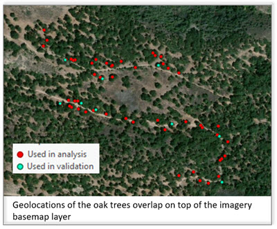
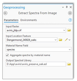
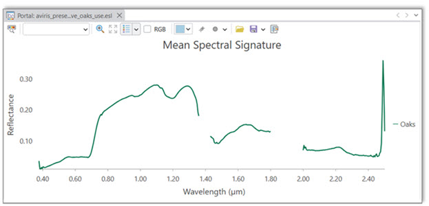
Using the Extract Spectra from Image tool, we extracted oak tree spectral signatures from the hyperspectral imagery at 51 field locations. We choose to aggregate the extracted spectra to create a mean oak tree spectral signature and save it as an Esri spectral library file (.esl).
We then shared the .esl file to ArcGIS Online as a spectral library item. The spectral signatures can also be viewed in ArcGIS Pro using the Spectral Signature Viewer.
Step 3: Calculate matching scores
We used the Detect Target Using Spectra service tool with the mean oak spectral signature in the spectral library portal item as the target. The tool compares the spectrum of each pixel in the hyperspectral imagery with the target signature and creates a tiled imagery layer containing the spectral matching scores.
In this workflow, we used the Spectral Angle Mapper (SAM) method. The output scores range from 0 to 1, with values closer to 1 indicating a closer spectral match to the mean oak signature.
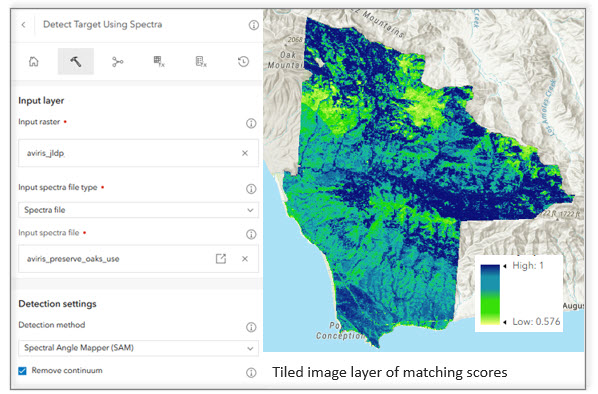
Step 4: Create the final oak tree map.
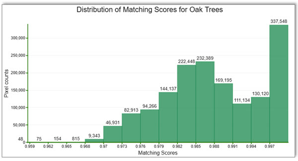
In this step, we identify pixels that closely match the mean oak spectral signature. The histogram of the matching scores in the web viewer shows a distinct peak near 1, corresponding to pixels with high spectral similarity to the target signature. Based on the histogram, we selected a threshold of 0.993 at the base of the peak to separate likely oak pixels from the rest of the image.
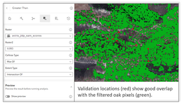
Using the Greater Than raster function, we applied the threshold to identify pixels with matching scores greater than 0.993. We then used the Preview option to visually examine the detected oak pixels together with the 9 validation locations that were set aside earlier. The selected threshold showed good overlap with the validation locations.
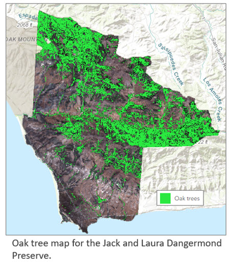
So we used this threshold and created the final oak tree map for the Preserve.
Note: There are several ways to filter pixels based on matching scores. In this workflow, we used the Great Than raster function because we have only one target. When multiple targets are used, the target detection output is a multiband raster, with each band containing the matching scores for a target, in this case, you can create a processing template to filter pixels for each band.
Summary
With the latest hyperspectral capabilities in ArcGIS Pro and ArcGIS Online, field observations and spectral libraries can be more easily incorporated into spectral analysis workflows and shared to the web. Together, these capabilities extend hyperspectral analysis beyond the desktop and provide an integrated workflow for creating, sharing, and applying spectral information for web-based image analysis.



Article Discussion: