The Greenland Ice Sheet is losing about 250 billion metric tons of of ice per year. It contributes to about 15% of total sea level rise from all sources each year. We now have various data sets and tools to measure the rate that elevations of land ice such as Greenland are changing. For example, the ICESat satellite, launched in 2003, was the first dedicated mission to measure ice sheet mass balance. Since then numerous satellite such as ICESat-2 and CryoSat-2 have also been launched specifically to measure ice surface elevations. Other sensors onboard satellites such as the Jason series, Sentinel-6 and SWOT can also be used to measure the elevation of land ice.
These sensors are collectively referred to as altimeters. Unlike traditional imaging sensors such as the ones onboard the Landsat series, altimeters send pulses of visible light or microwaves to the earth’s surface and measures the time it takes for the signal to return. Hence it is able to derive the elevation of the surface that the pulse hit.
Trajectory Dataset
Since the data from altimeters are stored as discreet points instead of images, we developed a new Trajectory Dataset to manage this type of data. Trajectory Dataset is similar to a Mosaic Dataset where it manages the measured points contained in the source NetCDF or HDF files. For each supported sensor, we developed a Trajectory Type to streamline the ingestion of source files to the Trajectory Dataset. We have 3 tools in the Trajectory Dateset Toolset: Create Trajectory Dataset, Add Data To Trajectory Dataset and Repair Trajectory Dataset Paths. With these tools you can extract relevant information from a source file for your analysis.
Use case: Greenland Ice Sheet
Here we are using the CryoSat-2 level-2 products to map the elevation of Greenland Ice Sheet from 2010 to 2021. This case will demonstrate a workflow that starts from adding data from multiple products and combining them for analysis, to creating an interpolated elevation dataset for each month, to generating a map of elevation change rate. The data is downloaded using the CryoSat User Tool provided by the European Space Agency.
Populating the Trajectory Dataset
First we create a new Trajectory Dataset using Create Trajectory Dataset:
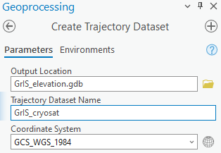
Then we use Add Data To Trajectory Dataset to add our downloaded files to the Trajectory Dataset. Choose Cryosat-2 as Trajectory Type.
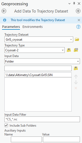
Very importantly, we need to open the Properties page of the Trajectory Type to further defined the product to want to add.

CryoSat-2 has 3 level-2 products corresponding to the 3 operation modes: SAR-Interferometry, Synthetic Aperture Radar and Low Resolution Mode. We need to specify the product we want using the Product Filter in the Trajectory Type properties page:
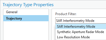
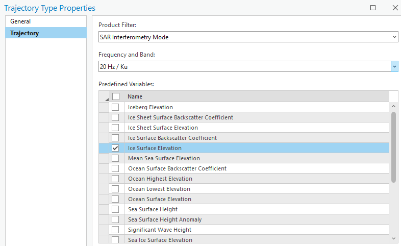
CryoSat operates in SAR-Interferometry and Low Resolution Mode over Greenland so we will choose SAR Interferometry mode first. We also need to choose 20Hz/Ku in Frequency and Band since most measurements are stored in the 20 Hz variables.
Then we have a long list of Predefined Variables that we derived from various fields in the source file. You can use them directly to get an analysis-ready Trajectory Dataset. This page documents how these variables are derived for each sensor and product. This is also a way to standardize field names in the Trajectory Dataset if you are using multiple sensors and the variable names are likely different for each sensor. For our case, we choose Ice Surface Elevation.
Alternatively you can import the native variables stored in the source file by specifying a sample file of the product you are adding.
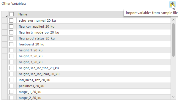
Once all properties are set, we can specify a Folder that contains all the source files. The tool will search for all files containing the SAR Interferometry measurements and populate with data that match the criteria.
Then we repeat this step and add data from the Low Resolution Mode. If you want to add even more data from other sensors such as ICESat-2, you can repeat the step again. Set the Trajectory Type as ICESat-2 and define the relevant product and variables in the Trajectory Type properties page. Everything will be contained within a single Trajectory Dataset.
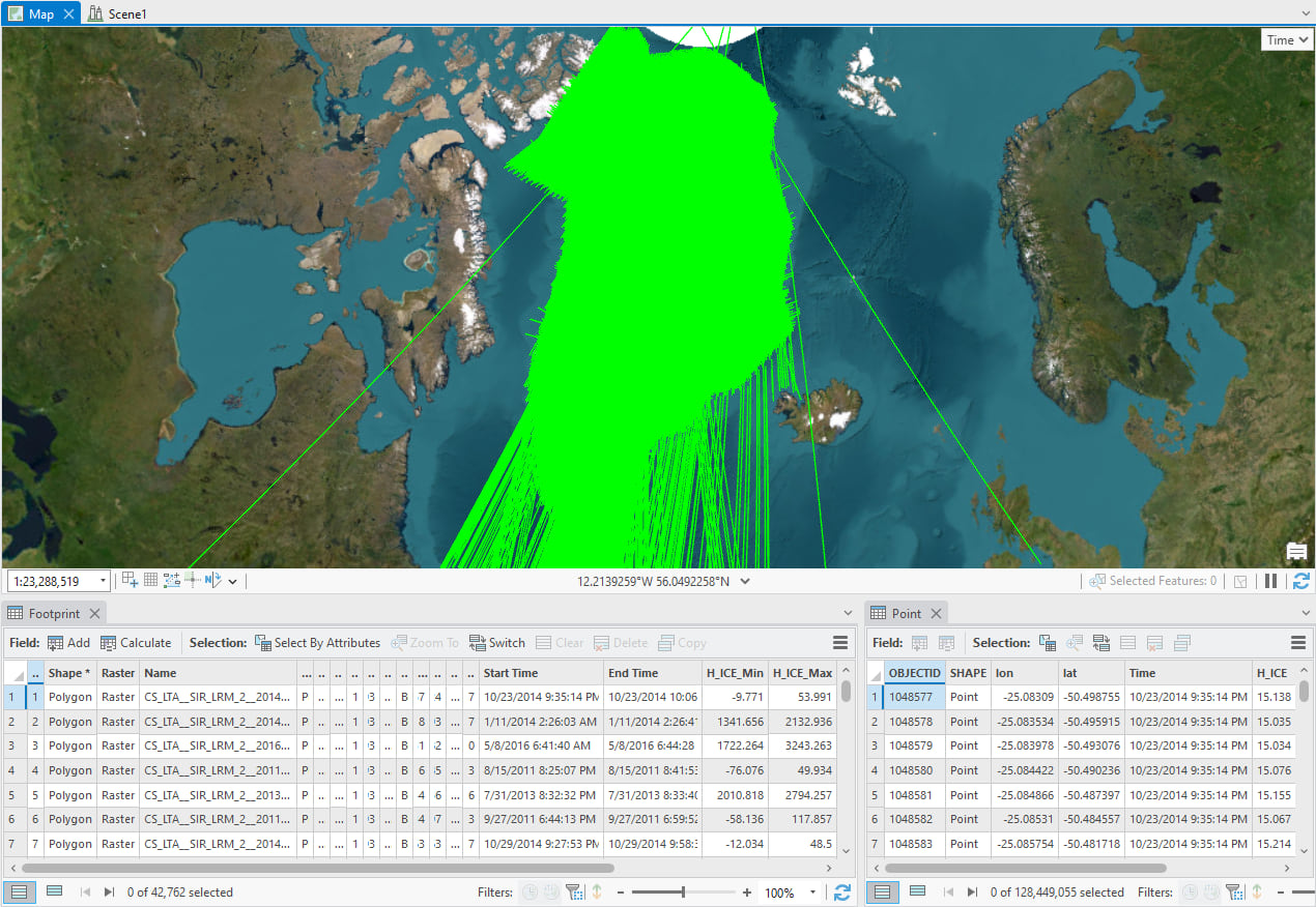
This is how our Trajectory Dataset looks like. It contains over 42000 tracks and 128 million points collected between 2010 and 2021. The Trajectory Dataset contains 2 sub-layers. The Footprint layer includes file names, start and end time of the track and maximum and minimum values of the included variables etc. The Point layer includes coordinates, collection time and any variable measurements that were defined in the Trajectory Type Properties page.
Performing analysis
After creating the Trajectory Dataset, we export the points of the Trajectory Dataset to a Point feature class. Then we use a Greenland Ice Sheet extent shapefile to remove points that lie outside of the ice sheet. We also remove obvious outlier points that have an elevation measurement below 0 m or above 3800 m. We are now left with about 65 million points.
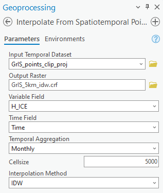
Then we use the Interpolate From Spatiotemporal Points tool to perform interpolation on these measurements. This tool is designed to work with points that have a time dimension as it can perform interpolation at specific time intervals. It automatically gathers points within temporal periods like Daily, Weekly, Monthly, Quarterly and Yearly, performs interpolation and output a multidimensional raster that contains interpolated results across the specified time periods. Here we specify the Variable Field as H_ICE, Temporal Aggregation to Monthly, Cellsize as 5000 and Interpolation Method as Inverse Distance Weighted (IDW).
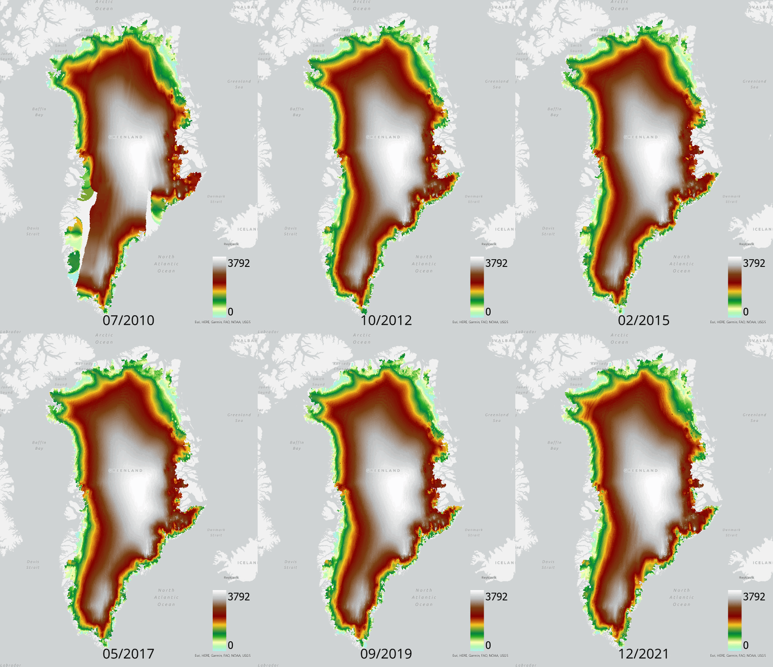
This produces a multidimensional raster at 5-km resolution representing the monthly elevation of Greenland Ice Sheet from 07/2010 to 12/2021.
Creating a map of change rate
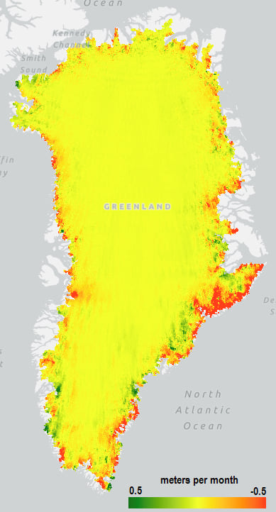
With the multidimensional output, we can use the Generate Trend Raster tool to estimate the change rate of Greenland Ice Sheet from 2010 to 2021. This is the map of elevation change rate derived from the Mann-Kendall method. The change rate is measured in meters per month estimated from Sen’s Slope.

Article Discussion: