ArcGIS GeoAnalytics Engine extends Apache Spark with a collection of over 140 spatial SQL functions and spatial analysis tools. It is a powerful python library that allows you to carry out your spatial analysis workflows within your Cloud platforms or on-premises Spark infrastructure.
In the demo for this year’s Developer Summit plenary, we leverage GeoAnalytics Engine within an Azure Databricks hosted PySpark notebook to perform custom big data analysis.
This demo identifies potential sites for new stores by investigating changes in consumer spending at brick-and-mortar stores throughout the United States. We used the Spend dataset from Esri partner SafeGraph. SafeGraph Spend is a points of interest (POIs) dataset providing anonymized, permissioned, and aggregated credit and debit transaction information. It includes date, time, location, details of businesses across the United States, as well as consumer spending metrics for online and in-person transactions. By joining spending data to Census Block groups, we can gain an understanding of how consumer spending behaviors change in different regions across the United States.
Prepare data and workspace
We used the following workflow to prepare the data and workspace:
- Create a Spark cluster in a cloud environment. For our demo we used Azure Databricks.
- Open a PySpark notebook.
- Import the geoanalytics and pyspark modules.
- Authorize GeoAnalytics Engine.
- Load the input Spend dataset into a PySpark DataFrame. We loaded our parquet dataset from Azure blob storage.
- Set location and time to enable the Spend dataset spatially and temporally.
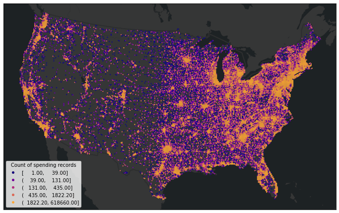
The Spend dataset used in this demo has 49 million spending records from January 1st, 2019 to January 1st, 2023. We can visualize the spatial distribution of the spending records by aggregating the data into bins.
Analyzing the change in in-person spending with US census block groups
To analyze the change in in-person spending at the block group level, we load the US census block group dataset from the Living Atlas into a PySpark DataFrame and then aggregate the spending records into block groups by calculating the total amount of in-person spending per year from 2019 to 2022. The table is pivoted for in-person spending in 2019 and 2022, and then we calculate the percent change in spending from 2019 to 2022.
# Aggregate the spending records to US census block groups
sg_spend_blocks = AggregatePoints() \
                  .setPolygons(block_groups) \
                  .setTimeStep(interval_duration=1, interval_unit="years") \
                  .addSummaryField("in_person_spend", "Sum", alias="sum_inperson_spend") \
                  .run(sg_spend)

# Calculate the percent change in in-person spending from 2019 to 2022
spend_blocks_pivoted = sg_spend_blocks.filter(F.col("COUNT") > 10).groupBy(blocks_fields) \
                           .pivot("step_start").agg(F.first("sum_inperson_spend").alias("inperson")) \
                           .select(blocks_fields + ["2019-01-01 00:00:00", "2022-01-01 00:00:00"]) \
                           .withColumn("inperson_pct_19_22", F.round((F.col("inperson_spend_2022") - F.col("2022-01-01 00:00:00"))/F.col("2019-01-01 00:00:00") *100, 2))
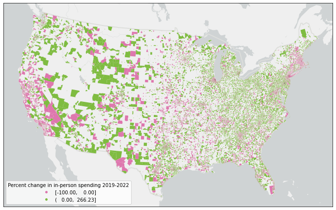
We next remove potential outliers. To find the outliers, we calculate the interquartile range (IQR) to find the difference between the third and first quartiles (Q3 and Q1) of the dataset. Any spending record with change that falls below the lower bound (Q1 – 1.5IQR) or above the upper bound (Q3 + 1.5IQR) is considered an outlier and removed from the spending dataset. Then we visualize the spatial pattern of the in-person spending change at the census block group level.
In this demo, we deployed the cluster with 10 workers running in parallel, which has 352 cores and 2816GB executor memory in total. It takes about 30 seconds to join the 49 million spending records within 240,000 block group polygons. We also tested with more data, to ensure this scaled. We simulated 1.5 billion spending records. Joining 1.5 billion spending records with 240,000 block groups completed on the same environment within 6 minutes.
Finding sites for new stores using the Find Similar Locations tool
As shown in Figure 2, in-person spending data is only available for some census block groups, but how can we evaluate every census block group to select suitable sites for a new store?
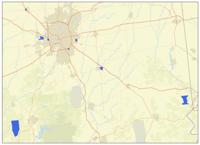
To answer that, we use the Find Similar Locations tool to find census block groups most similar to the block groups with the largest increase in in-person spending since 2020. The Find Similar locations tool requires a reference DataFrame, which represents what we want to match to. We create this by selecting ten top-performing census block groups, which are the 10 block groups with the largest increase in in-person spending after removing outliers. Second, we prepare both the reference and search DataFrames by choosing 40 economic and demographic variables relating to population, household, industry and income (e.g., Population Density, Average Household Size, Wholesale Trade, and Median Disposable Income) from the census block group feature service layer. To look for locations in the search DataFrame with similar demographics to the ten reference records, we run the Find Similar Locations tool to calculate cosine similarity (ranges from 1.0 for perfect similarity to -1.0 for perfect dissimilarity) among the census block groups. Figure 3 shows an example map of the potential block groups near Indianapolis, Indiana with cosine similarity index larger than 0.8.
# Select the 10 block groups with the highest averaged increase in spending from 2019 to 2022
top10_blocks = spend_blocks_cleaned.orderBy(F.col("inperson_pct_19_22").desc()).limit(10)

# Prepare the reference and search dataframes for similarity search
blocks_df = block_groups.select([F.col(item) for item in blocks_fields])
top10_df = blocks_df.join(top10_blocks, ["ID"], "inner").select(blocks_df["*"])

# Run Find Similar Locations tool for site selection, and get the similarity score
fsl_blocks = FindSimilarLocations() \
             .setAnalysisFields(*analysis_fields) \
             .setMostOrLeastSimilar(most_or_least_similar="MostSimilar") \
             .setMatchMethod(match_method="AttributeProfiles") \
             .setNumberOfResults(number_of_results=search_df.count()) \
             .setAppendFields("ObjectID", "Shape", "ID", "NAME", "ST_ABBREV", "STATE_NAME") \
             .run(reference_dataframe= top10_df, search_dataframe= blocks_df)
Conclusion
This demo showcases the power and versatility of the ArcGIS GeoAnalytics Engine for spatial analysis. By leveraging the SafeGraph Spend dataset and the US census block group dataset, we were able to gain insights into in-person spending patterns and identify potential sites for new stores using the Find Similar Locations tool. With the ability to process large amounts of spatial data quickly and efficiently, GeoAnalytics Engine can help businesses and organizations looking to make data-driven decisions. Refer to this PySpark Notebook for a detailed reference of the demo shown above.
To learn more about GeoAnalytics Engine, visit the GeoAnalytics Engine Guide and API reference. If you have any questions, please email us at geoanalytics-pes@esri.com.


Commenting is not enabled for this article.