Remote sensing is incredibly useful for informing us about things that we would have a hard time figuring out on our own, either because of high costs or difficulty accessing remote areas, or the time it would take to survey an area. But remote sensing can also tell us things that we already know, but don’t care to heed. For example, if you live in California, you’re experiencing one of the worst droughts in recorded history.
I have a couple of datasets here with really big pixels. One is a precipitation dataset which is 0.25 degrees and the other is NDVI at 4 km. Why use such big pixels you ask? These datasets represent two of the longest continuously collected series that we have, going back to the late 1970s. Big pixels show big patterns. If the pattern is big enough to be detected at 0.25 degree, then you have more confidence that it’s legitimate.
I talk about functions a lot in these blogs, but let’s not forget about the geoprocessing tools when working with imagery. There’s one in particular, Cell Statistics, which can be used in time series analysis. I’m going to use this tool to calculate the average precipitation and NDVI for all of the Octobers in each time series. Then, I’m going to use functions to subtract the average October from the October 2013 data for precipitation and NDVI and we’ll be able to see how this past October differs from an average October.
If you want to download the data, you can get it from these two sites: NDVI & Precipitation.
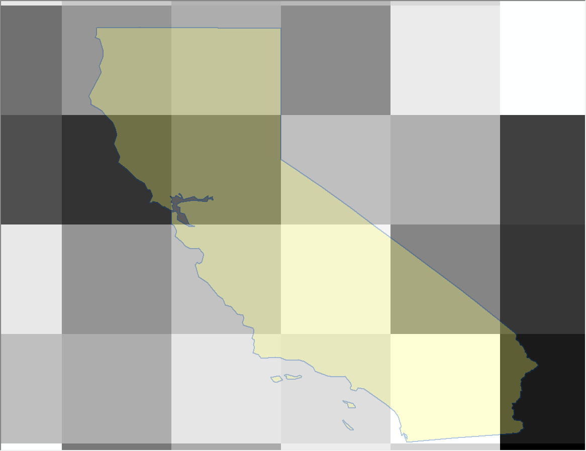
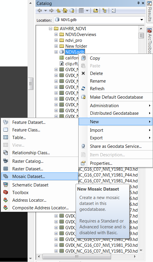
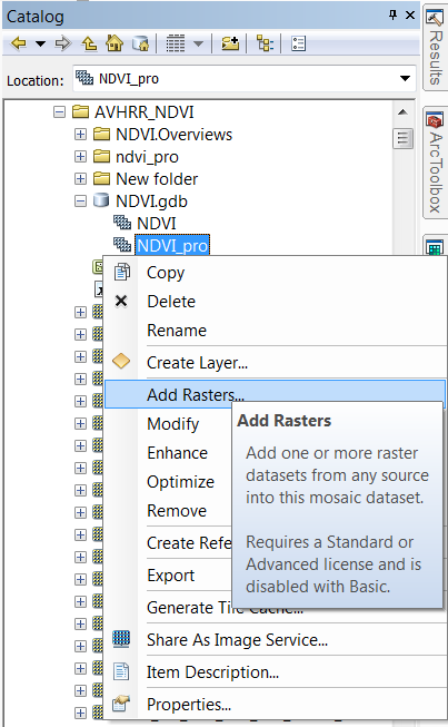
This image will give you a sense for how big these pixels are relative to the state of California. The first thing to do is to throw everything into a mosaic dataset. From Catalog, right click on a geodatabase, and create a new Mosaic Dataset. Once complete, right click on the mosaic and add rasters. Create separate mosaic datasets for precipitation and NDVI.
Having all of this data in mosaic datasets will become very useful later on because you can pull out only the time slices that you want to analyze. In this scenario, I’m only looking at October. The NDVI data comes weekly, so I’ve decided to use weeks 40 through 44 to represent October for each year. Precipitation comes in monthly time steps, so I just need to pick out every month 10 for each year.
From the Precipitation mosaic dataset, right click on the footprint, open the attribute table and make the selection for month 10. Then, right click again on the footprint and under Selection, choose Add selected rasters to map. This will allow you to create a group of just those rasters you have selected.
Open the Cell Statistics tool, populate it with the rasters from the group you just created, and fill in the remaining parameters. Make sure the overlay statistic is set to Mean. You get something like this:
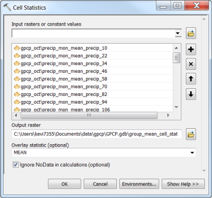
This will take all of the rasters you just threw at it, and calculate the mean value for each pixel over time. Do this for both precipitation and for NDVI. To get the October NDVI raster for 2013, you need to repeat this process with only weeks 40 – 44 selected from the year 2013. You don’t have to do that for precipitation.
Now, for the FUNctions part. ←See what I did there? Shameless.
Select the average October precipitation and the October 2013 precipitation rasters in the Image Analysis Window. Click the difference button. Repeat this for the average October NDVI and October 2013 NDVI. To create a region of interest, add a clip function on the resulting difference rasters. I’m applying a shapefile that I downloaded from ArcGIS Online of the state of California.
Here’s what you end up with after clipping. I’ve got my symbology set up so that negative differences are red, and positive differences are green. The yellow stuff is where there is minimal difference between this past October and the average October over the past 35 years.
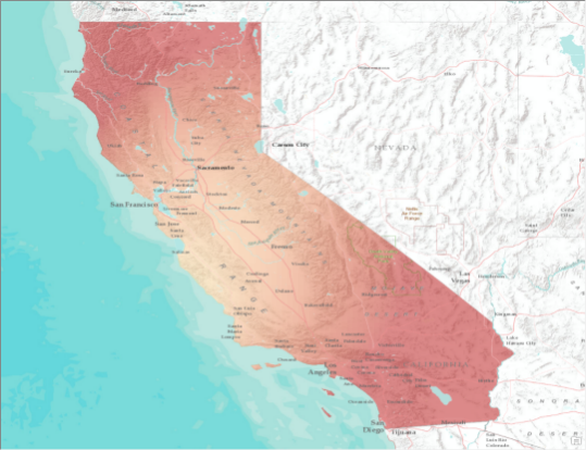
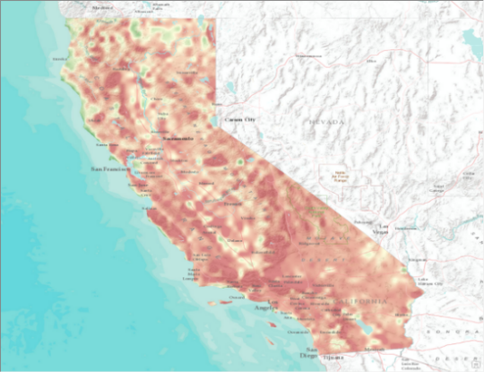
As you can see the northern and southern parts of the state were drier than average Octobers. What’s interesting is the NDVI map, which shows small pockets of higher than average NDVI. Some of this is actually the higher elevations, presumably snowpack that has melted prematurely, exposing the ground underneath. Water rights are complicated in California. Basically whoever claimed it first owns the rights in perpetuity, so that might explain some of the other pockets of higher than normal vegetation. Although the central valley had a fairly normal October, it’s expected to be dry there. They depend on water from the wetter, northern part of the state, which has been much drier than normal.
Article Discussion: