Previous tutorials in the 2019 winter and spring issues of ArcUser walked through an ArcGIS-based workflow that was used to successfully support a grant request by a district in Pierce County, Washington. This exercise measures the effects of the staffing increases made possible by the grant on the district’s response to emergencies.
This exercise uses actual response data, slightly filtered, to analyze more than six years of response activity for Graham Fire & Rescue (GF&R) to document the benefits of a grant it received in 2018.
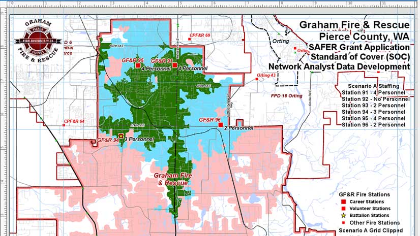
GF&R provides emergency fire, medical, and other services to Fire District 21 (FD 21), Pierce County, Washington. FD 21 is located in central Pierce County, approximately 20 miles southeast of Tacoma. GF&R protects more than 70 square miles of suburban and rural properties that have a population of more than 67,000.
From 2010 to 2019, the district’s population increased by nearly 20 percent, growing 3.4 percent in 2019 alone. FD 21 is one of the four fastest-growing large fire districts in Washington. In 2018, GF&R command staff recognized that the district’s growth was quickly challenging GF&R’s ability to provide quality essential services from its five staffed and one volunteer station. Planners note that annual emergency responses nearly doubled from 3,658 in 2010 to over 7,250 in 2019.
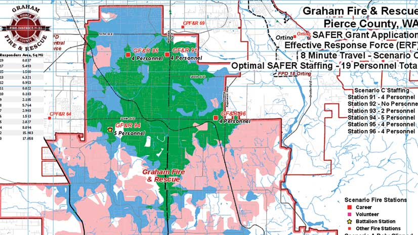
In April 2018, GF&R prepared and submitted a large request to the Federal Emergency Management Agency’s (FEMA) Staffing for Adequate Fire and Emergency Response (SAFER) grant program to expedite hiring of up to 21 line personnel and 5 new 24/7 firefighter positions. The $3.5 million grant, awarded in late summer 2018, provides 75 percent reimbursement for new personnel costs in the first two years and 35 percent reimbursement in the third year. The ArcGIS-based mapping and modeling that supported this grant request was featured in two ArcUser articles: “Mapping Current and Proposed Effective Fire Response” in winter 2019 and “Migrating Public Safety Workflows to ArcGIS Pro” in spring 2019.
The second year of the SAFER grant closed on August 31, 2020. As GF&R prepares annual performance reports, staff members have compiled more than six years of apparatus-level response data to support these reports. This data includes response type and travel times and staffing for all responding apparatus.
Getting Started
Tasks in this exercise include
- Review the SAFER program map
- Understand computer-aided dispatch (CAD)/record management system (RMS) data
- Import and map apparatus-level CAD/RMS data
- Modify tables to model emergency responder performance
- Create statistical summaries to measure and document performance changes
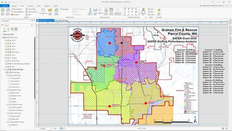
This tutorial expands on the two ArcUser tutorials previously mentioned. Begin by downloading the GFR_Maps sample dataset, unzip it, and store it on a local machine. Start ArcGIS Pro and navigate to \GFR_Maps\GFR_SAFER then locate GFR_SAFER.arpx and open it. This is essentially the same map created in the spring 2019 tutorial to compare the performance of the original fire station staffing and the staffing proposed if grant funds were received.
Study the four scenario staffing title boxes on this map layout to see the incremental changes. The scenario names include the staffing for each hiring interval and will be used to reference them. To measure the performance of these scenarios, you will compile and analyze changes in apparatus-level average travel time and staffing.
Before closing the layout, open the Bookmarks pane to see a single bookmark called GFR SAFER 1:80,000. If you become disoriented at any time in this exercise, use this bookmark to return to the full map extent.
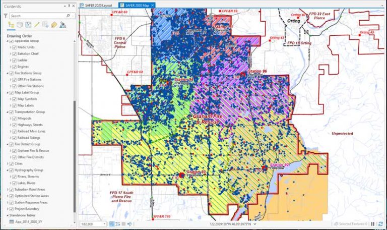
Switch from the Layout view to the Map view and study the map layers. Fire Station Group symbols show assigned apparatus and personnel in 2014, before SAFER hiring. The map also shows other important data layers including transportation, hydrography, assigned and optimized Station Response polygons, and Suburban and Rural classification.
Open the GFR Fire Stations attribute table to see all station location, apparatus, and personnel records. Review the current apparatus assignments and the staffing for each staffing interval. You will summarize all personnel and travel times for all responses within each time interval. You will test the premise that as staffing increases, more personnel arrive on scene, often in less time.
Introducing CAD/RMS Data
To perform this analysis, you will import more than six years of apparatus data, captured by the regional dispatch center and modified within GF&R’s record management system.
Save the project and minimize ArcGIS Pro. Use your file manager to locate and open APP_2014_2020_XY, the CAD data in a Microsoft Excel spreadsheet that is stored in \GFR_Maps\GFR_CAD_RMS. Inspect the spreadsheet and study all fields for 60,837 apparatus records from January 1, 2014, to May 5, 2020.
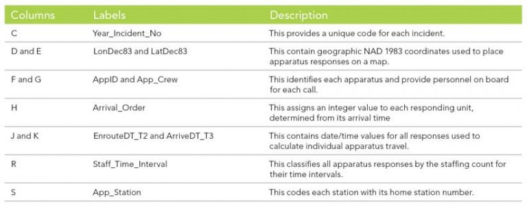
Table 1 includes CAD/RMS field names and a brief explanation of each field. Carefully review the columns in APP_2014_2020_XY as shown in Table 1. You will use many of these fields in this exercise.
The header names in this spreadsheet are field names that can be imported into ArcGIS because they all start with a letter; do not exceed 64 characters; and contain only letters, numbers, and underscores. All records and fields are formatted to properly import into a file geodatabase table.
Data Development and Management
Many agencies use Microsoft Excel spreadsheets to transfer data from dispatch to and through records management and onto a map. The CAD/RMS data for this exercise has been formatted and standardized to make the import seamless. The only records you will use will be ones with a travel time of 20 minutes or less. Sample data for this exercise has already been filtered to include only those records.
Close the spreadsheet without saving it and return to ArcGIS Pro then click the Analysis tab. In the search box of the Geoprocessing pane, type “table to excel” to locate the Excel To Table tool. Open it. In the wizard, set Input Excel File to GFR_Maps\GFR_CAD_RMS\ App_2014_2020_XY.xlsx. Set Output Table to App_2014_2020_XY and save it in GFR_Maps\GFR_Map_Data\Risk.gdb. (There is only one sheet so no need to select one.) Click Run to import the spreadsheet into your project. When the import is finished, open and inspect the table. Close the attribute table and save your project.
Creating and Symbolizing Apparatus Points
Creating apparatus data points in state plane coordinates is a two-step process.
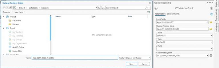
Step 1: On the Map ribbon, click Add Data and select XY Point Data. In the XY Table to Point geoprocessing tool wizard, select App_2014_2020_XY as the input table and store the Output Feature Class in \Risk.gdb, naming it App_2014_2020_X_GCS83. Set X and Y fields to LonDec83 and LatDec83. Click on the globe icon next to Coordinate System and choose Geographic Coordinate System > North America > USA and territories > NAD 1983 to set Coordinate System to GCS_North_American_1983.
In the Geoprocessing pane, click on Environments. Set the Output Coordinate System to GCS_North_American_1983 using the same process as previously described and click Run. Once it is finished importing, open the App_2014_2020_X_GCS83 attribute table and save your project.
Step 2: Export the GCS83 apparatus points to WA State Plane S. In Contents, right-click App_2014_2020_X_GCS83 and select Data > Export Features. In the Export Features wizard, verify App_2014_2020_X_GCS83 as Input Features, set the Output Location to Risk.gdb and Name the Output as App_2014_2020_X. Switch to Environment and use GFR Fire Stations to set the Output Coordinate System to NAD_1983_StatePlane_Washington_South_FIPA_4602_Feet and click OK.
After the apparatus points (i.e., App_2014_2020_X) load, remove App_2014_2020_X_GCS83 and open the new apparatus points attribute table.
In the Contents pane, right-click on App_2014_2020_X and choose Symbology. Click the three black bars in the upper right corner of the Symbology pane and choose Import Symbology. In the Apply Symbology From Layer tool verify App_2014_2020_X as Input Layer. Click the Symbology Layer browser, navigate to GFR_Map_Data, and select NFIRS All Responses. Set Source and Target fields as IncTypeNo and click Run. Save when the process completes.
Adding Important Fields
To measure staffing performance, you must add important fields: T3_T2, which will hold the travel time for all apparatus, and Response_Score, which will contain a rating of the response of apparatus. You will use ArcGIS Arcade, a scripting language for the ArcGIS platform, to perform interval time and response scoring calculations.
Inspect the attribute table for App_2014_2020_X and study the EnrouteDT_T2 and ArrivalDT_T3 fields. These fields contain complete date/time stamps for all apparatus records. You will add a new field and calculate the interval time between Enroute and Arrival times. In the Tables toolbar, select Add and in the Add Field Table, create a new field named T3_T2 and set its data type to Double.
Hint: You can use the Tab and Shift keys in combination to move between fields.
Add a second field named Response_Score and set its format to Double. In the Change area of the Field ribbon, click Save. Verify that your table contains the two new empty fields, close the Fields: App_2014_2020_X table, and save the project.
Calculating Fields Using ArcGIS Arcade
It is standard practice to calculate travel time in decimal minutes by simply subtracting date/time en route values from arrival times and multiplying the difference by 1,440, which is the number of minutes in a 24-hour day. This conversion is incorporated into the Field_Calculation_Scripts that has been included in the sample dataset for this exercise. This RTF file contains an ArcGIS Arcade script for calculating time interval and a Python script for calculating response scoring.
[To learn more about using Arcade for time calculation, see the accompanying article “Scripting Time Calculations in ArcGIS Arcade.”]
- In a file manager, navigate to GFR_Maps\Support, and open Field_Calculation_Scripts. Open it in Microsoft Word and float the window above or beside your project.
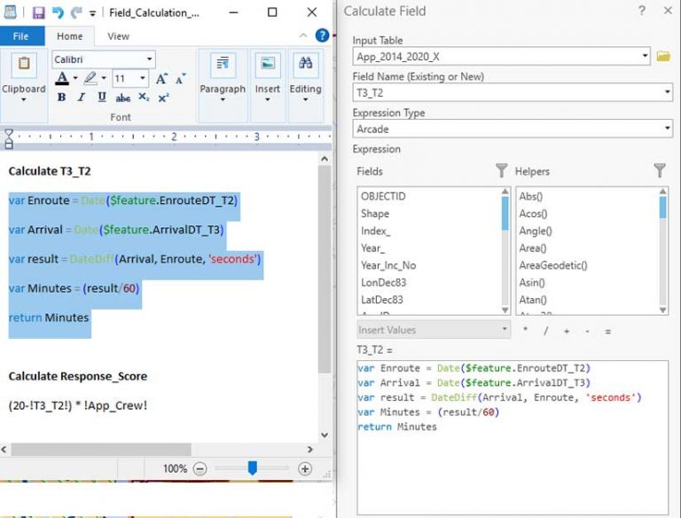
- Return to the App_2014_2020_X table, right-click on field T3_T2, and select Calculate Field. In the Calculate Field wizard, verify App_2014_2020_X as the Input Table and T3_T2 as the Field Name, and set Expression to Arcade. In Field_Calculation_Scripts, select the portion of the text under the heading Calculate T3_T2 and paste it into the formula box of the Calculate Field tool. Click Apply to calculate the travel time for apparatus in decimal minutes. Do not close the Calculate Field tool.
- Sort T3_T2 in descending and ascending order and inspect the data. Travel times will range from 0 to almost 20.
Creating One Performance Metric
You don’t need to close the Calculate Field tool because ArcGIS Pro supports multiple field calculations in one Calculate Field session. Now that you have travel times in decimal format, you can score each apparatus response based on the time that it took to arrive on scene. You can also track the personnel on each responding apparatus, so you can score arriving personnel, too.
Low travel numbers and high personnel counts (more firefighters on scene) represent good response. Since these values trend against each other, I decided to use a favorite geophysics trick from my dusty old geology toolbox, and invert one value before combining them. Since travel time is clipped by practice at a 20-minute maximum, I experimented with an inversion calculation of 20 minus travel time. I found that if I multiplied the inverted travel time by numbers of personnel on each arriving apparatus, I could easily quantify and display low response times and high personnel counts with a single value, the Response Score.
To calculate the Response Score, return to the Calculate Field tool and change the Field Name to Response_Score. Make sure that you change the Expression Type to Python 3. Remove the code for Calculate T3_T2 and replace it with one-line Response_Score script from Field_Calculation_Scripts and paste it into the text box under Response_Score =.
This script will subtract each travel time from 20 and then multiply the difference by responder count (the value stored in the App_Crew field).
Click OK to run this script and score all apparatus records. When it finishes running, sort Response_Score in ascending and descending order to verify that the field has been populated with values. Save the project.
Modeling Firefighter Performance Statistics
You will use the Response_Score, App_Crew, Time_Staff_Interval, App_Station, and AppID fields to summarize and measure apparatus-level response of four staffing intervals (Time_Staff_Interval). You can prepare multiple summaries for each responding station (App_Station) and for individual apparatus (AppID). This is a huge benefit because concatenated summarize-only fields are not required. (Also pivot tables are available only in ArcGIS Pro Advanced.)
You will prepare two multifield summary tables from the Response_Score field. ArcGIS Pro summary statistics support complex summaries across multiple fields. Note: Consistent table names are important.
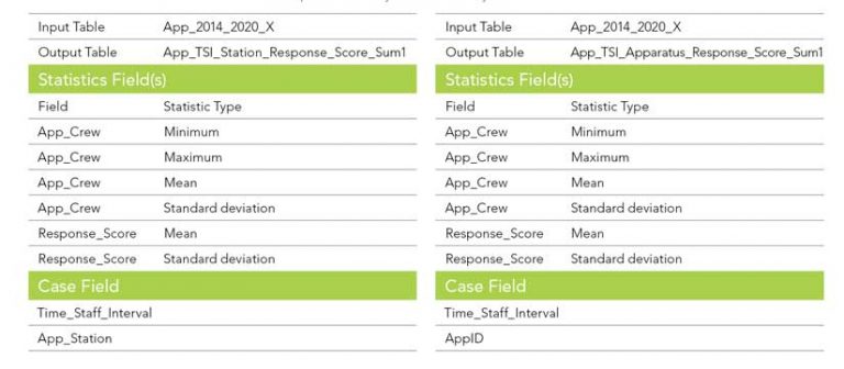
To measure station performance, you will create an App_TSI_Station_Response_Score to summarize data by personnel interval (Time_Staff_Interval) and station (App_Station). Return to the App_2014_2020_X table, right-click the Response_Score header and select Summarize. In the Summary Statistics wizard, set the parameters in Table 2 to create the summary table for App_TSI_Station_Response_Score. Be sure to store the Output Table in Risk.gdb. Click OK. The summary table for the stations is added to the bottom of the Contents pane. Save the project.
To measure individual apparatus performance, you will summarize data by personnel interval (Time_Staff_Interval) and apparatus (AppID). Right-click on the Response_Score header and select Summarize then use the parameters in Table 3 to create the summary for App_TSI_Apparatus_Response_Score. Store the Output Table in Risk.gdb. Click OK. The summary table for the apparatus is added to the bottom of the Contents pane. Save the project. Close the Summary Statistics wizard, and save the project.
Measuring the Effects of Staffing Changes
These summary tables will help you see how changes in the staffing of GF&R stations affected their response in terms of time and number of apparatus.
Open both summary tables you just created and stretch them to show at least 24 records. In App_TSI_Station_Response_Score_Sum1, right-click App_Station and select Custom Sort. Define a Custom Sort so that App_Station sorts first and Time_Staff_Interval sorts second, both in ascending order. Click OK.
Highlight Stations 91, 93, and 95. Look at the values for Mean_App_Crew and Mean_Response_Score. Review all stations and focus on Stations 94, 96, and 91, the three stations that received SAFER personnel.
On September 1, 2018, two new personnel were assigned to Station 94 during Time_Staff_Interval (TSI) 17. Note that its mean App_Crew decreased slightly from Interval 15 to 17, increased during TSI 19, and decreased slightly through TSI 20.
Mean_Response_Score increased through TSI 17 and 19, falling slightly during TSI 20. Headquarters/Battalion Station 94 supports operations throughout the district and a moderate increase is not unexpected.
Two SAFER firefighters began service at Station 96 on September 1, 2019 (TSI 19). Mean_App_Crew and Mean_Response_Score increased slightly in TSI 17 and significantly in TSI 19, falling slightly in TSI 20. With two additional crew assigned in TSI 19, Station 96 soon experienced a significant performance improvements during TSI 19.
The fifth SAFER firefighter was assigned to Station 91 on January 1, 2020 (TSI 20). Station 91 is often GF&R’s busiest station, housing the district’s ladder, a reserve engine, and a medic unit. The SAFER firefighter increased staffing for Station 91 to five, with three firefighters on the ladder and two on the medic unit. The values for Mean_App_Crew and Mean_Response_Score for Station 91 increased during TSI 17 and 19. During TSI 20, the staffing score increased slightly and the response score was flat.
Looking at Selected Summary Apparatus Data
Click App_TSI_Apparatus_Response_Score_Sum1, right-click on AppID, and select Custom Sort. Create a two-field sort referencing AppID, followed by Time_Staff_Interval, both in ascending order. After sorting, open Select By Attributes from the Table frame. In the Select By Attributes wizard, create a new expression that selects all Station 91 apparatus by limiting records to those with AppID containing the text 91.
Run this query, and now you see all Station 91 apparatus, grouped in ascending Time_Staff_Interval. Check apparatus staffing and response scores for units. Notice that Engine 91 (E91) responds only occasionally, with Ladder 91 (L91) performing most duties. The new firefighter was assigned primarily to L91, so the mean staffing and response scores increase.
Modify your attribute selection to show all equipment responding from Station 94. Both activity and staffing increased slightly for E94 in TSI 17 and 19 but decreased slightly in TSI 20. M94 shows slight continuous increase through all periods. The battalion chief (BC94) typically responds alone and shows a slight score decrease in TSI 20. Note that the Brush unit (BR94) responds only occasionally and typically with a crew of two.
Finally, change the selection query to show only Station 96. This station shows a considerable increase in staffing and performance during TSI 19, with two new SAFER firefighters. Staffing and scores decreased slightly in TSI 20.
Look at station and apparatus summaries for the three other GF&R stations. You may observe some rather unusual trends in TSI 20. For a quick explanation, GF&R initiated a COVID-19 operations plan on March 15, 2020 that included separating the service area into two battalion areas. With some detective work, you can identify and map pre- and post-COVID-19 activities by apparatus and station.
Save your project.
You are finished!
Summary and Acknowledgments
In this detailed and comprehensive exercise, you used actual response data from Fire District 21, a quickly growing fire district in suburban Pierce County, Washington, to assess and report improvements that resulted from funds provided by a SAFER grant program. This tutorial tells just part of the story.
Special thanks to the command staff at Graham Fire & Rescue for providing me with the chance to prepare and present this interesting tutorial. Thanks also to Esri Technical Support for introducing me to time-based calculations in ArcGIS Arcade.