From suggesting how many steps we should walk in a day, to predicting the future price of our home, machine learning (ML) is becoming an integral part of our lives. ML is a new approach to understanding our universe based on exposing data-driven relationships and predicting outcomes without empirical models. Here at Esri, we are focused on empowering our users to unlock the full potential of their data using The Science of Where. The intersection of GIS and ML is a new frontier for turning spatial data into deep spatial understanding, and there are so many ways to integrate these powerful technologies to answer seemingly unanswerable questions. We recently did an analysis to predict global seagrass occurrence by harnessing the commonly used ML libraries of sci-kit learn and spatial analysis power of ArcGIS.
Why do we care about seagrass?
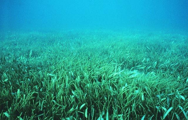
These bottom-attached marine plants play an important role in combating global warming, storing up to 100 times more carbon-dioxide compared to tropical forests. Despite their importance, travelling to every shallow part of the ocean to check for seagrasses is a gargantuan undertaking. We would like to build a data-driven model of seagrass occurrence which can be useful if we want to understand its role in the global ecosystem.
How can we predict where seagrass is growing?
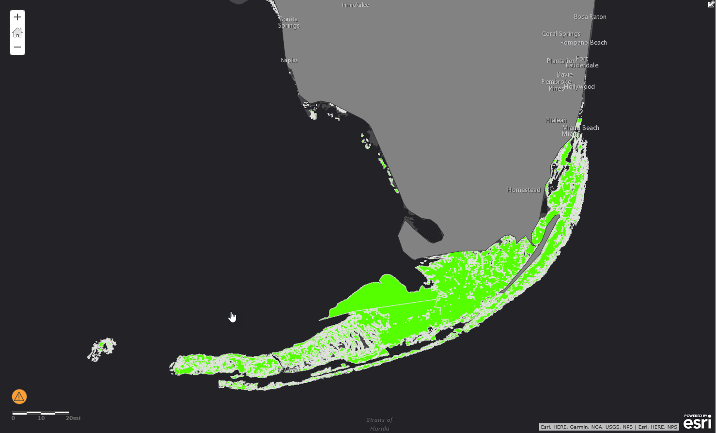
Bottom-attached seagrasses occur in shallow coasts around the world. We know some of the general characteristics of where they live, things like ocean temperature, salinity, and the content of various minerals and nutrients, and we have global data for each of these characteristics from the Ecological Marine Units dataset. Luckily, we also have detailed seagrass data from the U.S. Marine Cadestre that is publicly available for the entire U.S. coast, which will act as our training data. The general workflow will be to: 1) accurately estimate ocean conditions in between measured values, 2) build a machine learning model for a subset of the data for the U.S. coast using a Random Forest classifier, 3) test of accuracy of the model using the remaining data, and 4) predict global seagrass occurrence.
Using EBK to create a truly global dataset
Global data on oceanic conditions (like temperature, salinity, minerals and nutrients) is available at discrete locations, but our goal is to predict seagrass occurrence at any location in the ocean. So, we started the analysis with Empirical Bayesian Kriging (EBK), a powerful spatial analysis tool in ArcGIS, to interpolate discrete measurement data on ocean conditions into statistically valid continuous surfaces. Creating this continuous, global dataset allowed us to train the model that predicts seagrass occurrence from ocean conditions all along the U.S. coast, and ultimately predict seagrass anywhere in the world.
Predicting Globally
Now that we have all the data that we need, we’ll use Random Forest classifier to model the relationships between oceanic conditions and seagrass occurrence. You can follow along with the entire analysis, as well as get more details about decisions behind methods, parameters, and more, in the Jupyter notebook we used to perform the analysis, taking advantage of the arcpy package (another great option for this kind of integration is the ArcGIS API for Python)
Since the next step of our analysis is to use a Random Forest classifier to predict seagrass occurrence globally, we thought it would be useful to describe, at least conceptually, what that really means in the context of our analysis.
Random forests use decision trees for classification and forecasting. They are a very widely used technique within ML as they require a small number of input parameters, which makes them approachable by most.
An illustration of a decision tree for classification in the context of seagrasses is given below:
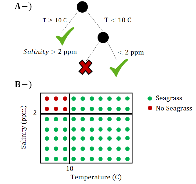
The training data for the illustration above shows that seagrasses always grow if water temperature is more than 10 C. However, if the water temperature is less than 10 C, then salinity has an effect on seagrass growth. Although classification trees provide a flexible and powerful way to perform prediction and classification, they generally suffer from over-fitting the data. That means that they do a great job predicting with the exact dataset being used, but have trouble when being used to predict or classify other data. Random forests address this limitation by creating many decision trees to randomly sampled subsets of the data. Thus, instead of one classification tree there are multiple trees used to perform classification. Note that the actual analysis uses decision trees that incorporate additional variables to the analysis
The first step of our Random Forest analysis was to train the model using a subset of the U.S. seagrass occurrence data, and then test the model’s performance using the remaining data. We were thrilled to see that our results show 97.8% accuracy!
Note: Even with an accuracy of 97.8%, we need to think about the applicability of the model we built to the entire dataset. Just like any other statistical model, Random Forests have their limitations. Although they are powerful interpolators, they are poor extrapolators. Thus, we cannot accurately predict areas where oceanic conditions fall outside the bounds of U.S. coastal conditions. To deal with this limitation, we eliminated areas close to the Poles that fell outside of the bounds of the training data.
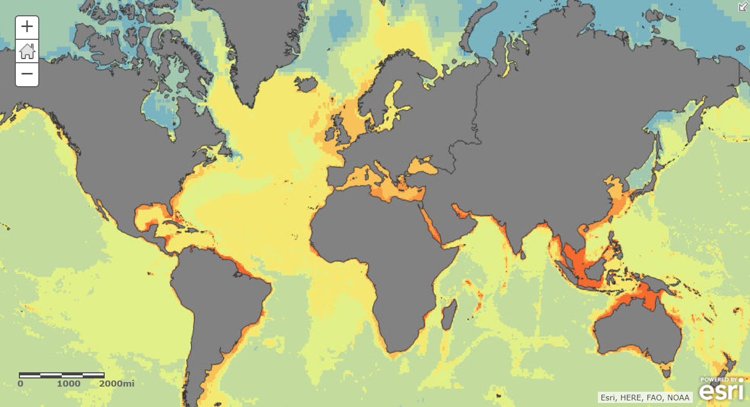
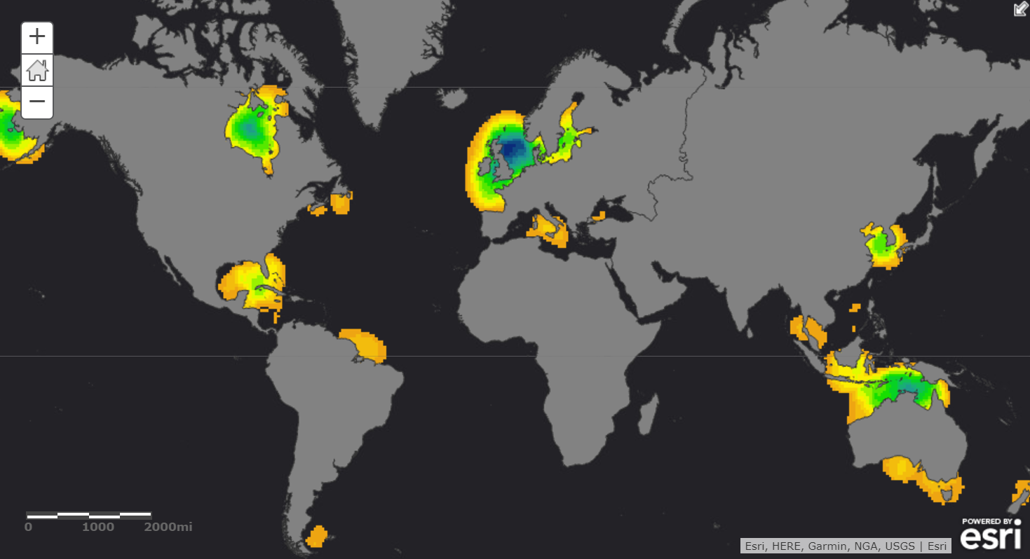
Finally, we made our prediction, and in order to better understand the spatial pattern of seagrass occurrence, we created a density surface based on the results.
The intersection of GIS and ML
This workflow illustrates the power of bringing together GIS and ML to tackle complex spatial problems. The intersection of GIS and ML is full of opportunities to gain spatial understanding of complex problems, taking advantage of the immense amount of spatial and spatiotemporal data being collected within our organizations and around the world. We’re actively working to build the tools that help you integrate existing methods and technology, as well as pushing the limits of what it means to make machine learning truly spatial.
References
- Larkum, A. W. D., & Den Hartog, C. (1989). Evolution and biogeography of seagrasses. Biology of seagrasses. Elsevier, Amsterdam, 112-156.
- Duarte, C. M., Borum, J., Short, F. T., & Walker, D. (2008). Seagrass ecosystems: their global status and prospects. In Aquatic ecosystems: trends and global prospects (pp. 281-294). Cambridge University Press.
- Short, F., Carruthers, T., Dennison, W., &Waycott, M. (2007). Global seagrassdistribution and diversity: a bioregional model.Journal of Experimental Marine Biologyand Ecology,350(1), 3-20.
The blog post is provided by Orhun Aydin. Orhun is a product engineer in the Spatial Statistics team. You can reach Orhun at OAydin@esri.com

Article Discussion: