In this blog post, I share some information about one of the world’s strangest and most wonderful landform features—the curvaceous and mesmerizing braided river valley of Russia’s Ob River. I also explain how I was able to reveal its hidden nature through maps.
For other interesting terrain revelations, keep watching this ArcGIS Blog.
Ob River
According to Encyclopaedia Britannica: “One of the greatest rivers of Asia, the Ob flows north and west across western Siberia in a twisting diagonal from its sources in the Altai Mountains to its outlet through the Gulf of Ob into the Kara Sea of the Arctic Ocean.”
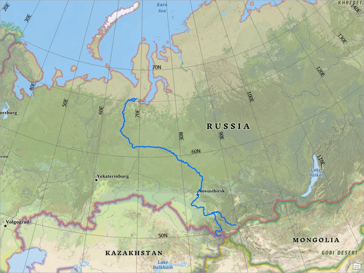
According to Amusing Planet, the Ob River in western Siberia, Russia, is the world’s seventh-longest river. Although the “real” length of a river is a subject that is often disputed (see, for example, the debate about the world’s longest river according to Live Science), the Ob River is indisputably one of the world’s longest rivers.
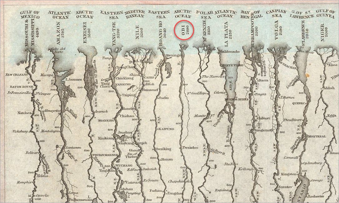
This beautiful 1849 historical map by G. Woolworth Colton also claims that the Ob River is the seventh-longest river in the world . . .
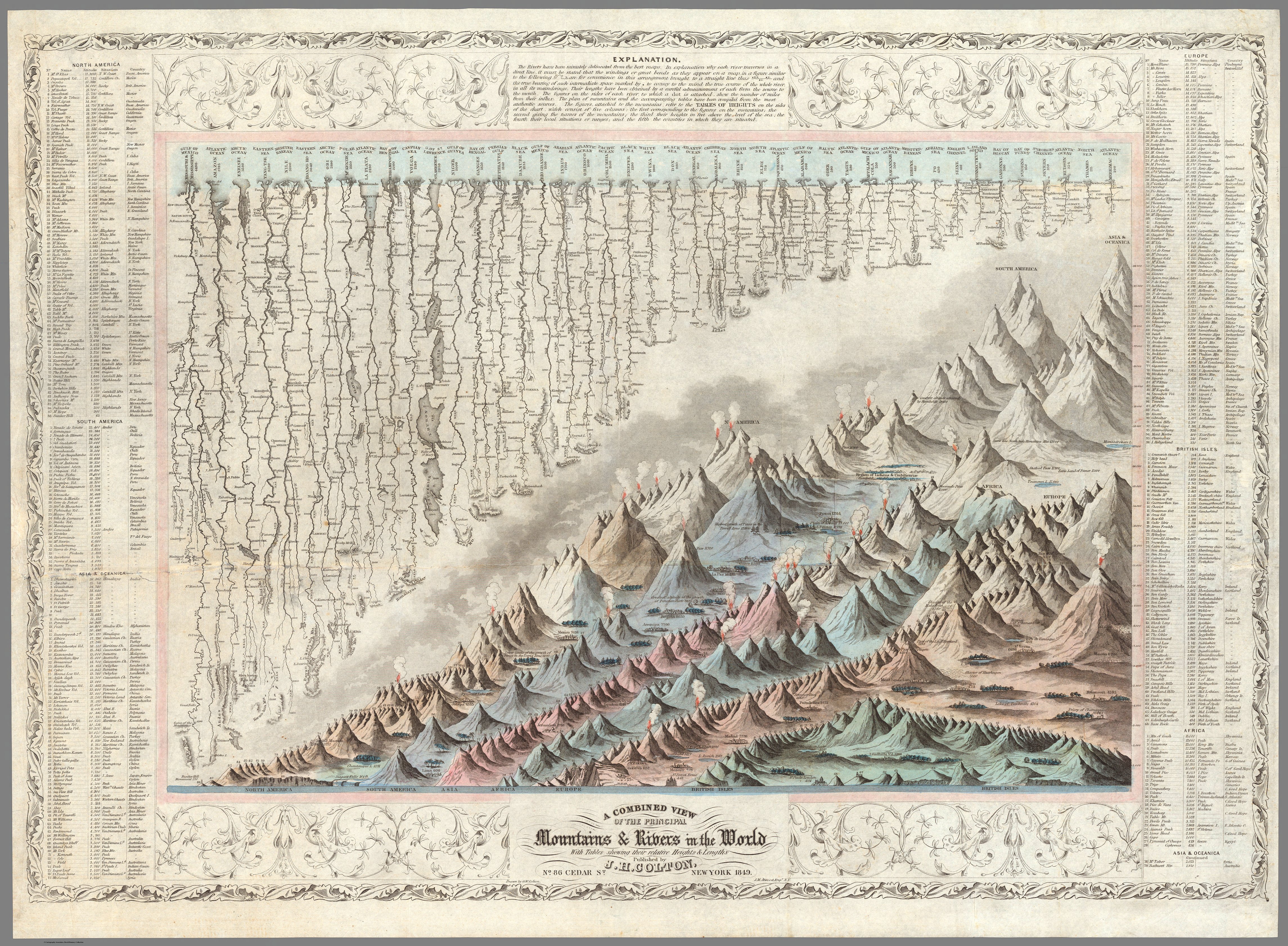
(Image source: https://www.davidrumsey.com/luna/servlet/detail/RUMSEY~8~1~1644~130003:Mountains-&-Rivers–Published-by-J-?trs=57&mi=36&qvq=mgid%3A2151)
. . . which can clearly be seen in this close-up of the map.
Doing a little research in the Encyclopaedia Britannica, I learned: “In its course through the taiga, the middle Ob has a minimal gradient, a valley broadening to 18 to 30 miles (29 to 48 km) wide, and a correspondingly broadening floodplain—12 to 18 miles (19 to 29 km) wide. In this part of its course, the Ob flows in a complex network of channels, with the main bed widening from less than 1 mile (about 1 km) on the higher reaches to nearly 2 miles (3 km) at the confluence with the Irtysh and becoming progressively free of shoals.”
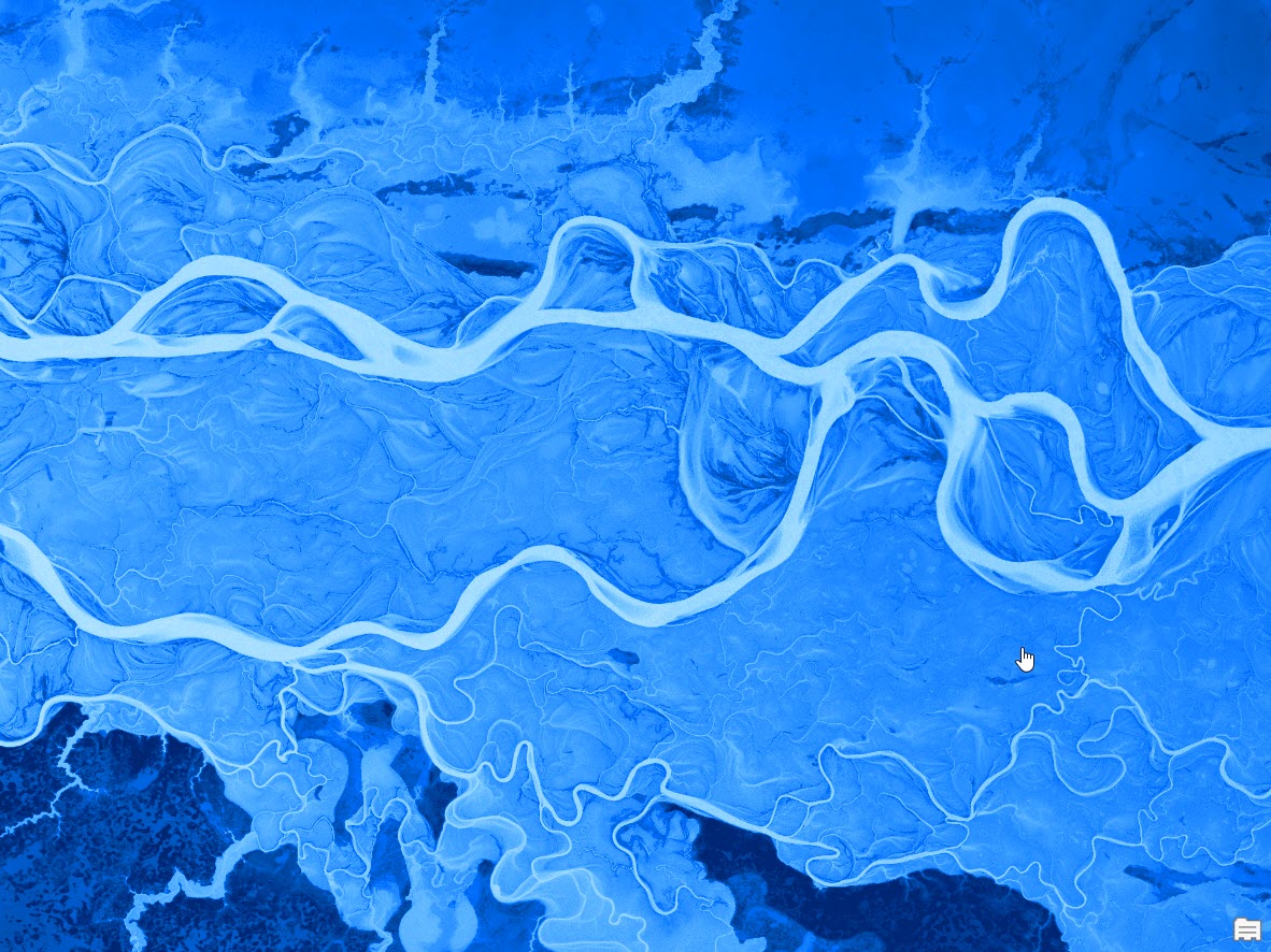
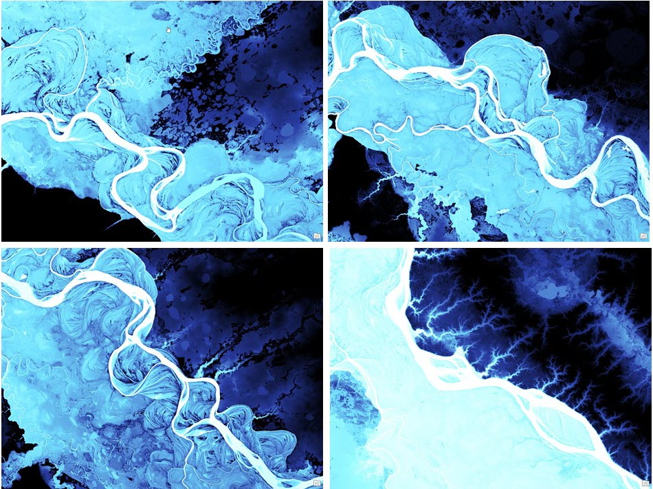
I was especially interested in the area where the river’s floodplain was wide and the river meandered freely. I knew this was where the river flow would be slow and there would be a buildup of sediment in the river valley. Like other braided rivers, side channels and temporary islands would be created and re-created as the water flowed largely unobstructed across the extensive, flat landscape.
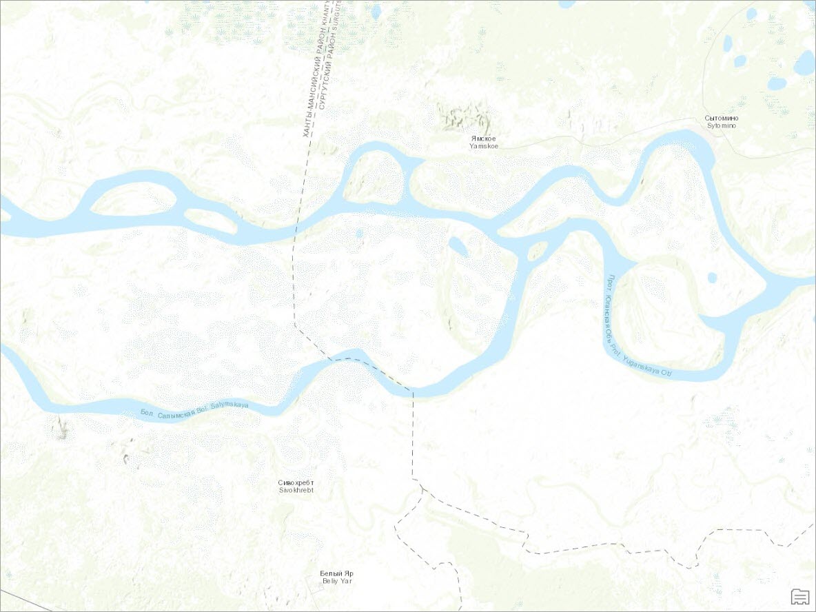
So I focused on an area (shown by the red dot on the map below) in the West Siberian Plain to the east of the confluence of the Irtysh River (shown in lighter blue) and Ob River.
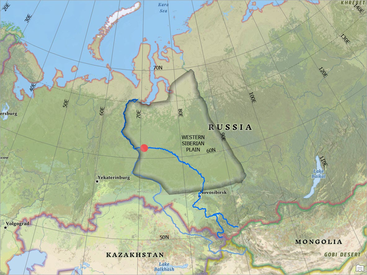
(Data source for the 1:10,000,000 scale Geography Regions polygon: Natural Earth.)
Maps
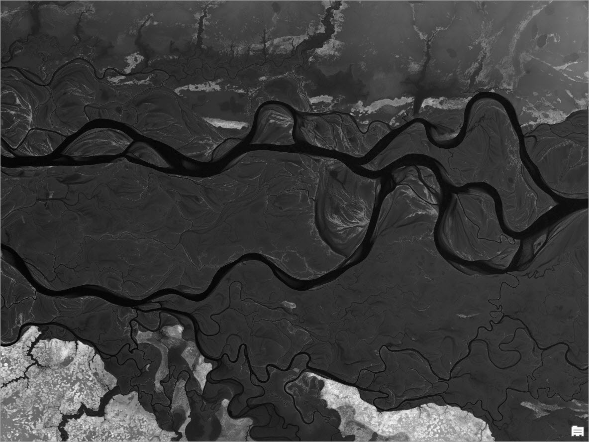
Exploring the ArcGIS Topographic Basemap didn’t really reveal what I had expected.
Here’s how I unveiled the concealed beauty of the braided river valley using nothing more than the Terrain imagery layer from ArcGIS Living Atlas of the World and varying a few settings in ArcGIS Pro.
First, I added the Terrain imagery layer and used the Dynamic Range Adjustment (DRA) feature to make sure that the display was being rendered using the statistics from the pixels in the view, not the whole dataset. To do this, click the Appearance tab and click the DRA button or select this option from the Statistics drop-down menu in the Symbology pane. Note: It is best to use the DRA feature in ArcGIS Pro 2.1 or later versions.
This is almost always the first thing I do when I add the Terrain layer to any map, because it shows much more variation in the display. As you pan and zoom, the display updates automatically to use information about the pixels in the new view. Already I could see more details about the river than the topographic map revealed.
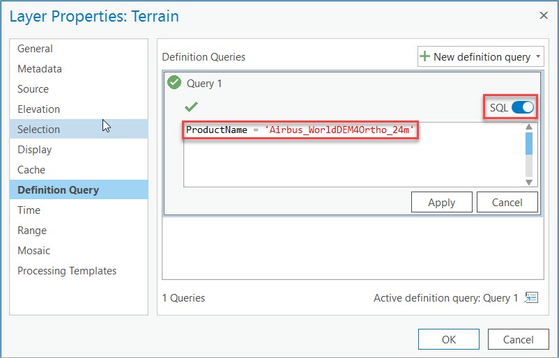
Making sure I was visualizing the higher-resolution Airbus data in the Terrain layer was even easier than ever now that the required definition query is shown in the pop-up pane.
Ensure that the map scale is less than about 1:430,000. Click the Terrain layer in the map view. You’ll see in the top of the pane that multiple elevation data sources are available at this map scale. Click the WorldDEM_WDO_08_N61_00_E0710_00_DEM data source. Note: in the bottom of the pane, you’ll see that this elevation source has a resolution (i.e., pixel size) of about 25 meters. Copy the SQL query at the bottom of the pane to your computer clipboard.
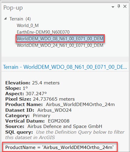
Right-click the Terrain layer in the Contents pane, click the Definition Query tab, and add a new definition query. Click the SQL toggle switch, paste the SQL query, click Apply, and click OK.
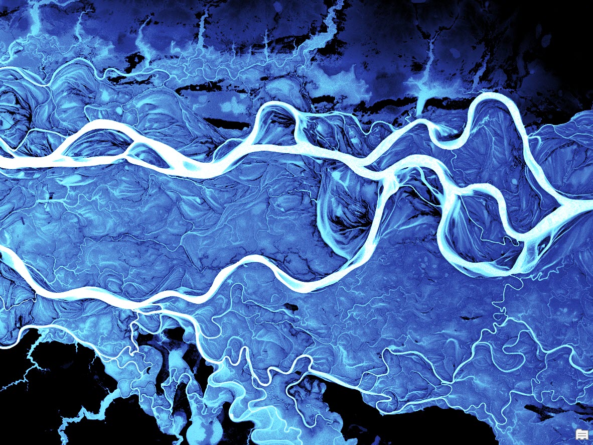
Next, I started working with the symbology. In the Symbology pane, I chose the Bathymetry 4 color scheme.
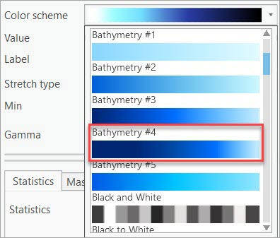
Since the bathymetry color schemes were created to range from dark blue for lower values (that is, deeper waters) to light blue for higher values (or shallower waters), the first step was to invert the color scheme. To do this, click the color scheme, choose Format color scheme, and click the Invert button  .
.
In the Symbology pane, I changed the Stretch type to Percent Clip stretch with the Min set to 1.0 and the Max set to 12.0.
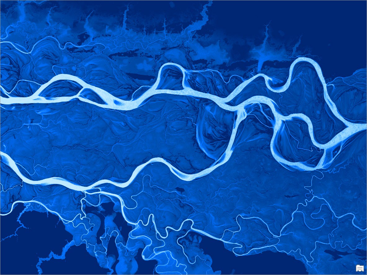
This made fewer of the pixels with the lowest elevations appear lighter, and more of the pixels with higher values appear darker.
To make the river pop out and add some variation in the middle elevation areas, I modified the Bathymetry 4 color scheme. In the Symbology pane, click the color scheme, click Format color scheme, and edit the properties in the Color Scheme Editor. Note: if you like what you end up with, you can click the option to Save to a style.
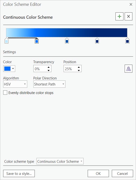
I changed the end colors to white and black, deleted the dark blue color (second from the right), moved the lighter blue color a little to the left, and added some cyan to the range of lighter colors. To really make the river pop out, I added a second white color near the end.
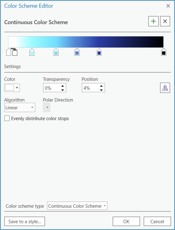
The result was the map you saw earlier in this blog post. Because the color scheme is applied to the entire Terrain layer and the DRA feature ensures that the statistics of the current view are used to render the map, you can pan around to find other interesting locations the spellbinding landscape.
Remember that the Airbus data is viewable up to map scale of about 1:430,000, so zooming out beyond that map scale will make the Terrain layer disappear from view.
Hopefully, you will find use for these methods to reveal the complex terrain features that are sometimes hidden in our landscapes. Watch for upcoming blog posts to see other interesting places I’ve found and learn how I mapped them. Spoiler alert: Some of these are noted in my earlier blog post Introducing Terrain Revelations.


Commenting is not enabled for this article.