A century ago, the boll weevil spread across the American South, decimating its cotton crops. The US State of Georgia was compelled to diversify its agriculture. What other crops could Georgians grow instead? They needed a new strategy.
At about the same time, rail cars with refrigeration started to bring fresh fruit to new markets. Peaches became a crop that helped Georgia diversify its economy. Georgia earned a new nickname, the Peach State.
But how many acres of peach orchards still remain in Georgia 100 years later? Does the nickname still apply?
Let’s use ArcGIS Pro and the ArcGIS Living Atlas of the World and find out.
First, open ArcGIS Pro and start a new project.
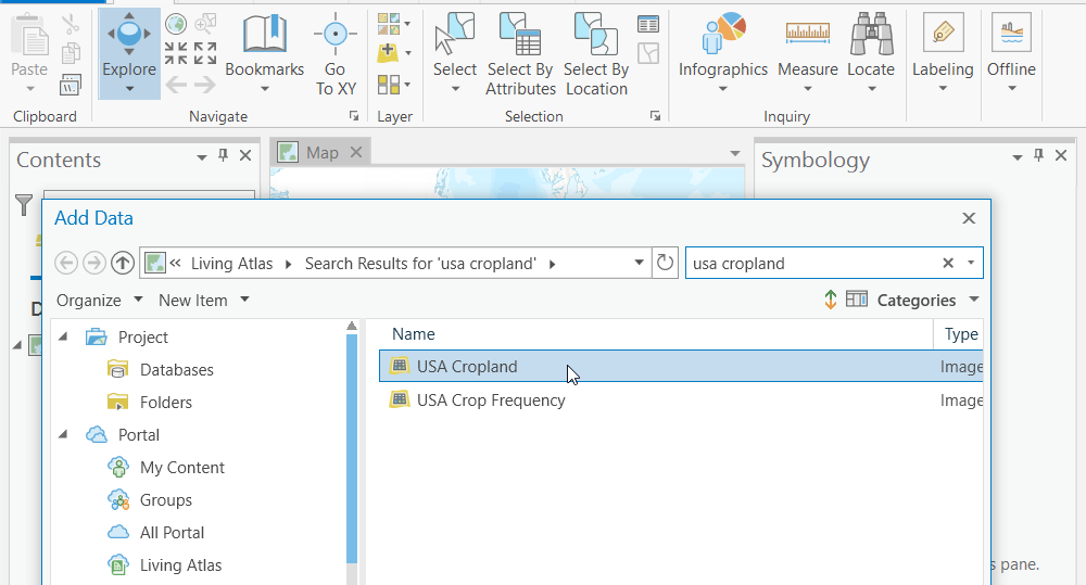
In the map ribbon, click on ‘add data’. Then in the dialogue that comes up, click on living atlas on the left, under portal. We’re going to search for the ‘USA Cropland’ layer in the living atlas. USA Cropland is a time enabled imagery layer of the USDA CropScape Cropland Data Layers dataset from the National Agricultural Statistics Service (NASS). In the box in the upper right, type “cropland”. You’ll see the USA Cropland layer from the Living Atlas in the window, click on it, and click ok.
Now let’s add the states. Click on ‘add data’ again, then click on the living atlas tab again to search just living atlas layers. In the box on the upper right type ‘states’. You will see the feature layer “United States State Boundaries 2018”, click on it, and click ok to add it to your map.

We have two layers in our map. Now let’s make sure we use the most recent crop year for our analysis, and use just the State of Georgia instead of all 50 states. We do this by applying a definition query to each layer. For states, we want to make sure the only state we use for analysis is Georgia. To do this, right click USA_State in the table of contents, and choose properties. On the tabs on the left choose definition query. In the dialogue, click new definition query. Choose ‘STATE_NAME’ on the left, ‘is equal to’ in the center, then choose Georgia from the list. Now click apply, then OK.

We are going to use this shape (for the state of Georgia) to clip out a piece of the cropland layer later, and to do this, we need the shape to be in the same projection as the raster layer USA_Cropland. To do this, we’ll make a copy of the state. Choose the analysis ribbon along the top, and click the tools button. In the geoprocessing pane, search for the tool ‘copy features’. In the parameters dialogue, choose USA_State for the input features. For output feature class, type ‘Georgia’.

In the environments tab, where it says output coordinate system, choose the same coordinate system as USA Cropland, which is Albers conical equal area projection. You always want to perform raster analysis in an equal area projection if you want an accurate count of area in your result table. Now click run.

Now that we have Georgia, let’s make sure the data for the cropland is current. By default the layer displays all years from 2008 to 2019 so it can be played in an animation. But we want to know how many acres of peaches are grown in Georgia in the most current year available. Let’s set a definition query so that we choose only the year 2019 in our layer.
To do this, Right-click on USA Cropland in the table of contents, then choose properties. Then click on the definition query. Next, make a definition query that says ‘ProductName’ on the left, ‘is equal to’ in the center, and ‘2019’ on the right. Now click apply. Click OK.

Optional: Apply a processing template that filters out only the fruit crops (including peaches) in the service. Let’s choose the ‘Fruit’ processing template to logically filter the service so that the result contains only fruit crops. To do this, right-click on ‘USA Cropland’ in the table of contents, then choose properties. At the very bottom, click on processing templates. On the right-hand side, you will see the processing template is the analytic renderer. With the dialogue, find the ‘fruit’ template and click ‘ok’. Now your output table will only have fruit crops.

Now that we have a polygon for Georgia and the cropland layer set to 2019, we are ready to make a table of how many acres of the different kinds of crops (including peaches) were grown in Georgia.
To do this we will use the extract by mask tool in spatial analyst. On the top ribbon choose the analysis tab, and under that, click the button for tools. The geoprocessing pane will appear on the right. Type ‘extract by mask’ and then hit enter in the tool to search. Click on the extract by mask tool in the search results.

The extract by mask dialogue has two tabs, the parameters and the environments tab. Let’s work on the parameters side first. Where it says input raster, choose USA Cropland. Where it says input raster or feature mask data, we’ll choose the feature ‘Georgia’. Provide a name for the output raster, or use the suggested name (probably Extract_USA_1).

Now let’s enter some values in the Environments tab. I like to have my table output a pixel count in acres, so I’m going to have my analysis resample to a cellsize that is exactly one acre. To do this, where it says cell size, enter the value 63.615. This is the square root of 4046.86, which is the number of square meters in an acre. Now click run.

Extract by mask takes a minute to run, but when it’s done you will see a new raster in the table of contents called Extract_USA_1. Right click Extract_USA_1 in the table of contents and choose attribute table. The count field shows the number of pixels of each crop (and each pixel is one acre). My result for peaches was 18,089 acres.

Further investigation:
How many acres of peaches were grown in Georgia in 2009 (ten years ago)? What’s the difference in acreage between then and now?


Article Discussion: