Have you tried to use near real-time GIS data in your analytical tools, such as tracking a hurricane, assessing areas affected by an earthquake, or mapping flooded areas during a storm? ArcGIS Living Atlas of the World contains a collection of near real-time layers known as Live Feeds. Live Feeds display the latest information available such as active hurricanes, recent earthquakes, or river streamflow forecast. Moreover, these layers can be used in analytical tools, connecting Live Feeds to real-time analysis of current conditions, such as interactively mapping flooded areas for first responders in Austin, Texas.
Utilizing near real-time data in analytical tools often requires the automation of tools and workflows that can run with minimal maintenance or supervision, which can sometimes be challenging. The good news is the development of these tools is easily done using Python. In this blog, I’ll show how to consume Live Feed data from Living Atlas through the ArcGIS REST API and the ArcGIS API for Python using two examples: acquiring river streamflow forecast data and plotting changes in arctic sea ice extent.
Retrieving data from Living Atlas through the ArcGIS REST API
ArcGIS Online items, such as the items in Living Atlas, contain a REST service endpoint which can be leveraged by the ArcGIS REST API. The ArcGIS REST API allows us to interact with the items’ service to query, subset, and retrieve Live Feed data. The Live Feed data returned from the interactive request can be seamlessly included in web apps, workflows and more.
Let’s explore how we can retrieve forecasted river streamflow data from the National Water Model.
Access the REST endpoint
Go to the Living Atlas webpage and search for “National Water Model.”

Select the “National Water Model (10 Day Forecast).”
")
On the item’s overview page, scroll to the bottom. The endpoint is in the URL box at the bottom-right corner. Click on “view” to open it in a new tab.

The item contains only one layer: “Flow Forecast (cfs)”. Click on it to access the REST endpoint. The webpage displays all the relevant metadata such as extent, time info, and field names. At the bottom, click on “query.”
The query webpage contains boxes to interactively construct a request. Alternatively, we can use the endpoint (i.e. url) https://livefeeds2.arcgis.com/arcgis/rest/services/NFIE/NationalWaterModel_Medium/MapServer/0/query to construct the query string and request the data.
Example: Query forecasted river streamflow data for a single reach of the National Hydrography Dataset (NHD)
We’ll plot the forecasted streamflow for Onion Creek in Austin, Texas. The station ID (i.e. COMID) of Onion Creek in the National Hydrography Dataset (NHD) is 5781733. We can query the forecast for this creek by adding the parameter:
where=egdb.dbo.LargeScale_v2.station_id=5781733Additionally, we can request (1) to include all fields, (2) order the results by time, (3) return a maximum of 80 records, and (4) to return the data in JSON format.
outFields=*&
orderByFields=egdb.dbo.medium_term_current.timevalue&
resultRecordCount=80&
f=pjson
The query url is constructed as follows:
https://livefeeds2.arcgis.com/arcgis/rest/services/NFIE/NationalWaterModel_Medium/MapServer/0/query?
where=egdb.dbo.LargeScale_v2.station_id=5781733&outFields=*&
orderByFields=egdb.dbo.medium_term_current.timevalue&
resultRecordCount=80&f=pjson
The requested data is returned in json format.

Note: You can load the results in ArcGIS Pro using the JSON to Features tool and create Line Chart.

Example: Query forecast streamflow data for an area
We’ll subset the National Water Model (NWM) forecast data for South Austin. We provide the following parameters: (1) the subset area geometry, (2) the geometry type, (3) the spatial relationship, and (4) the time stamp 2019-07-22 09:00:00 (i.e. 1563786000000).
geometry={xmin:-10889680,ymin:3524030,xmax:-10873880,ymax:3537115}&
geometryType=esriGeometryEnvelope&
spatialRel=esriSpatialRelIntersects&
time=1563786000000
The query url is:
https://livefeeds2.arcgis.com/arcgis/rest/services/NFIE/NationalWaterModel_Medium/MapServer/0/query?
where=&
time=1563786000000&geometry={xmin:-10889680,ymin:3524030,xmax:-10873880,ymax:3537115}&
geometryType=esriGeometryEnvelope&
spatialRel=esriSpatialRelIntersects&
outFields=*&
resultRecordCount=50&
f=pjson
Note: We are requesting data from a Live Feed layer in which the Time Extent changes frequently. The time selected in this blog post won’t be available after the hosted layer is updated. You can select a different time that falls within the current Time Extent. The current Time Extent and Time Interval can be checked in the REST endpoint and also in the Return Updates operation.

The requested results for the forecast time of 2019-07-22 09:00:00 at South Austin are shown next.

Note: You can quickly transform time expressions from datetime variables to milliseconds from 1970-01-01 and vice versa as follows:

Note: The ARGIS REST API documentation includes a complete description on how to query a feature service.
Accessing Living Atlas data using the ArcGIS API for Python
Living Atlas items are also available through the ArcGIS API for Python. The layers can be queried, plotted, and used in analytical workflows. In addition, we can leverage the ArcGIS API for Python through ArcGIS Notebooks.
Let’s examine how Arctic Sea Ice Extent has changed over time.
Example: Plot the changes in arctic sea ice extent in September
Open an ArcGIS Notebook in ArcGIS Enterprise or in your desktop.
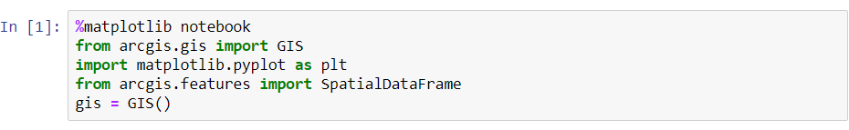
Load the required modules.
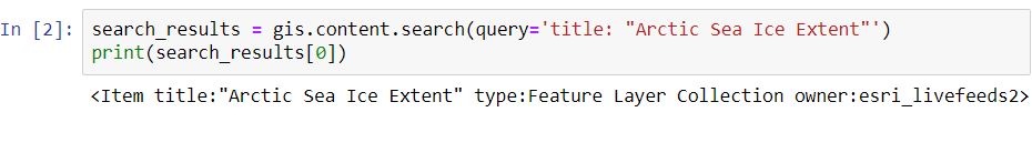
Search for the ‘Arctic Sea Ice Extent’ item.
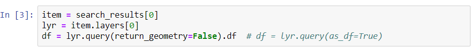
Select the first layer and query the data as a DataFrame.
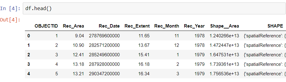
Visualize the structure of the data set by plotting the top rows.
Subset the DataFrame by selecting only the months of September for all years.

Plot all months of September in the data set.
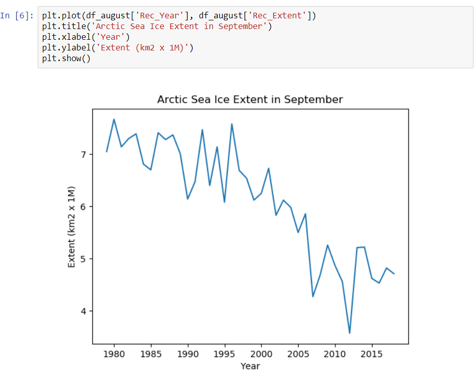
The python script used in the example will query all the monthly data in the Arctic Sea Ice Extent feature service. As soon as new monthly values are added to the service, those can be queried and plotted with the same python script.
Summary
The ArcGIS Living Atlas of the World includes Live Feed layers that can be queried, subset, and retrieved systematically in analytical workflows using the ArcGIS REST API and the ArcGIS API for Python.
Related Learn ArcGIS resources
- Update Real-Time Data with Python: Learn more about how to create your own Live Feed.
More Information?
Join GeoNet and ask a question to our community of experts.

Commenting is not enabled for this article.