With the latest release of ArcGIS Pro 2.9, many new and improved capabilities are now available for your spatial statistical workflows. These include a new tool called Presence-only prediction, a new tool called Change Point Detection, and Fields Statistics to Table tool. In addition, various enhancements to the existing Data Engineering view, Fill Missing Values tool, Spatial Outlier Detection tool, and Forest-based forecast tool will help improve your analysis workflows. Let’s look at each of them in more details!
Are you a researcher wanting to understand the impact that climate change will have on the habitat of a sensitive species?
Are you a flood hazard analyst who wants to estimate the probability of flooding following a hurricane landfall or an epidemiologist wanting to model the emergence of new infectious diseases?
Are you a wildlife ecologist with field data for observed presence locations of a plant species and want to estimate the species’ presence in a broader study area?
Are you interested in learning predictive analytics?
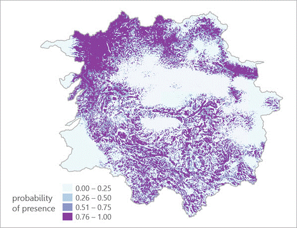
If your answer is yes to any of the above questions, then you should check out the new Presence-only Prediction (MaxEnt) geoprocessing tool in ArcGIS Pro 2.9. The tool estimates the presence of a phenomenon in a study area using previously known presence locations and explanatory factors.
The Presence-only Prediction uses a maximum entropy approach (MaxEnt) to estimate the probability of presence of a phenomenon. The tool uses known occurrence points and explanatory variables in the form of fields, rasters, or distance features to provide an estimate of presence across a study area. You can use the trained model to predict presence in different data if corresponding explanatory variables are known. Unlike other methods that either assume or explicitly require defined absence locations, Presence-only Prediction can be applied to prediction problems where only the presence of the event is known. This tool is available in the Spatial Statistics Toolbox (Modeling Spatial Relationships toolset).

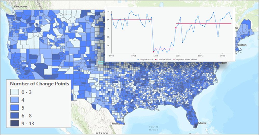
The tool detects time steps when a statistical property of the time series changes for each location of a space-time cube. Identifying important changes in a time series can be widely applicable to all walks of life from weather and climate monitoring, monitoring COVID-19 daily cases or estimating flu seasons across locations, monitoring advertising campaign impacts to urban planning and so on.
For each location in a space-time cube, the Change Point Detection tool identifies time steps when some statistical property of the time series changes. The tool can detect changes in the mean value or standard deviation of continuous variables, as well as changes in the mean of count variables.
The change points divide each time series into segments, where the values within each segment have a similar mean or standard deviation. The number of change points at each location can be determined by the tool or a defined number of change points can be provided that is used for all locations. This tool is available in the Space Time Pattern Mining Toolbox (Space Time Pattern Analysis toolset).

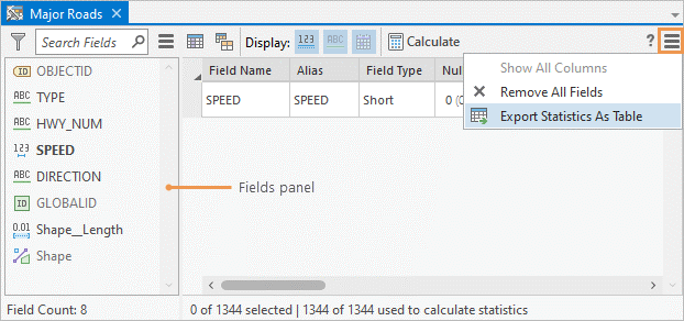
The tool creates a table of descriptive statistics for one or more input fields in a table or feature class and is available in the Data Management Toolbox (Fields toolset). To help understand your data better, the tool outputs all the relevant statistics for the input field by default. You can choose to customize the output tables and statistics for different field types. For example, you can specify separate output tables to store all the numeric and date fields in addition to only selecting the statistics of interest.
This tool is complementary to the Data Engineering view introduced in ArcGIS Pro 2.8. The available statistics for each field type are the same as those available in the Data Engineering view. For a complete list of supported statistics and how each statistic is calculated, see Interact with statistics.
4. Data Engineering view (new features & improvements)
The Data Engineering view, released with ArcGIS Pro 2.8, helps you explore, visualize, clean, and prepare your data quickly and confidently. In ArcGIS Pro 2.9 we have focused on quality of life improvements and bug fixes to make your Data Engineering experience better. At the top of the list are these 5 enhancements:
- Any easy button to export the Data Engineering statistics as table using the Field Statistics to Table tool.
- A new feature to open the attribute table for the field of interest – no more scrolling through hundreds of fields in the attribute table to find the field you’re interested in!
- Easy access to Data Engineering view from Fields View and Attribute Table.
- Drag one or more fields from the fields panel into geoprocessing tool parameters that accept input fields.
- Quick access to the count of number of fields in the layer, as well as a count of the number of fields matching a filter or search criteria.

5. Forest-based Forecast (new Multivariate forest-based forecast)
The Forest-based Forecast tool forecasts the values of each location of a space-time cube using an adaptation of Leo Breiman’s random forest algorithm. The tool has been enhanced in ArcGIS Pro 2.9 which now includes the ability to incorporate explanatory variables in the forecasts and estimate lagged effects between the variables. Other explanatory variables can be provided to improve the forecast of the analysis variable, and you can estimate and visualize lagged effects between the explanatory variables and the variable being forecasted.
If any other variables are provided, the forecast model is a multivariate forest-based forecast. Each explanatory variable is converted to time-lagged factors within each time window that are used to train the forest model. This allows you to estimate any lagged (delayed) effect between the explanatory variables and the analysis variable. For example, a rise in the number of COVID-19 hospitalizations may predict the number of deaths 14 days later.
6. Spatial Outlier Detection (new Global outlier detection method)
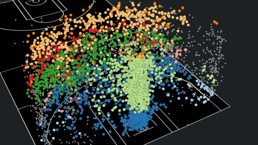
As the name suggests, the tool identifies spatial outliers in point features. In ArcGIS Pro 2.9, the tool has been enhanced to detect global spatial outliers in addition to local spatial outliers. A global outlier is a point that is far away from all other points in the feature class. A local outlier is a point that is farther away from its neighbors than would be expected by the density of points in the local area. With this enhancement, you will have more control over the definition of an outlier for the problem you’re trying to solve.
For example, a map of emergency rooms across a state may identify emergency rooms in low population areas as global outliers because there are larger distances between them compared to high population areas. However, for the same example of emergency rooms in a state, a local spatial outlier is a hospital that is far from other emergency rooms, taking into account the changing density of the emergency rooms across the state. This could identify emergency rooms in high population areas that service more people than surrounding emergency rooms, which could identify areas with lower access to emergency care.
7. Fill Missing Values (now supports stand-alone tables)
Fill missing values tool is one of the most widely used Spatial Statistics tool to replace missing (null) values with estimated values based on spatial neighbors, space-time neighbors, and time-series values. The tool has been enhanced to fill missing values in stand-alone tables. For stand-alone tables, the missing values can be estimated using global statistics of the input field or time-series values. For example, if you have the U.S. county-level data in a table, you can fill the missing values using the average of all the counties in the same state.


Article Discussion: