Isolated geographic coordinates (latitude and longitude) lack descriptive context. Unless you’re familiar with geographic coordinates, raw numbers like these don’t tell you much. Is this a city, a forest, a desert, or a mountain? Humans recognize places by their surroundings, not their coordinates. A satellite image instantly reveals buildings, roads, farmland, snow, water, or forest. To make coordinates more meaningful, location embeddings represent these numbers in a rich description of the surrounding physical environment.
Understanding location embeddings
Before understanding a location encoder, it helps to understand the concept of an embedding. An embedding is a compact numerical representation that captures the important characteristics of something, for example:
- A person’s face can be represented by a vector that captures facial features.
- A sentence can be represented by numbers that capture its meaning.
- An image can be represented by numbers describing its visual content.
Similarly, a geographic location can be represented the same way: instead of storing only latitude and longitude, a stored learned vector summarizes what makes that place unique. This is a location embedding.
What a location encoder does
A location encoder is a deep learning model that converts coordinates into these embeddings. Rather than treating coordinates as just numbers on a map, it learns the environmental and geographic characteristics tied to various locations across the globe so places with similar landscapes (forests, farmland, deserts, coastlines, cities, and so on) produce similar embeddings, even across different countries.
For example, given only the coordinates 34.0564 degrees north, 117.1956 degrees west, a computer has no context about the physical landscape. A location encoder processes these coordinates into an n-dimensional embedding, something like [0.22, 0.79, 0.41, …, n] that encodes the environmental attributes of that area. Since computers can’t see a map the way a human can, this translation step is what gives raw coordinates structured, usable meaning.
Esri has developed location encoding models, each designed to capture different aspects of geographic information. These include the USA Geodemographic embeddings created using Geodemographic Foundation Model (GDFM), which is trained on demographic data, and the Global Location Encoder (Sentinel-2), which is trained on Sentinel-2 satellite imagery. Because these models are built on different architectures and trained on different data sources, they capture different representations of geographic locations.
Why location encoding matters in GIS
The encoder learns a continuous function over geographic space. Locations that are environmentally similar but far apart—such as two temperate rainforests on opposite sides of the world—can end up close together in embedding space, while neighboring locations with very different land cover may end up far apart. Spatial proximity in the real world doesn’t equal proximity in embedding space; ecological similarity does.
By learning the relationship between coordinates and satellite imagery, the location encoder captures the environmental and physical characteristics of a region. The Esri Global Location Encoder (Sentinel-2) model is based on SatCLIP architecture and is trained on 2024 globally distributed Sentinel-2 Level-2 imagery using 12 bands of the 13 bands (it does not use B10) . Learn more about how to use Global Location Encoder (Sentinel-2) model.
From coordinates to insights
The workflow typically follows a structured path from raw data to a usable GIS product:
- Embedding generation—Geographic coordinates (latitude, longitude) are used as input in the pretrained Global Location Encoder (Sentinel-2) model. The model processes the coordinates through neural network layers to produce a fixed-length vector.
- Downstream task—These vectors are used as features in traditional GIS tools or machine learning models.
- Visualization—The results are mapped back into a GIS environment to show clusters, heatmaps, or predictions.
Use and apply the model with tools
Location embeddings support a range of downstream tasks—such as similarity search, clustering, and geospatial data enrichment and improve predictive modelling tasks like classification and regression. Traditionally, identifying areas with similar geographic characteristics whether for mineral exploration, land cover mapping, or environmental monitoring has relied on manually engineered indices, threshold-based classification, or time-intensive expert interpretation. The Generate Embeddings Using AI Models and Find Similar Features Using Embeddings GeoAI tools offer a different approach. The first uses deep learning to derive location embeddings that encode the underlying spatial, spectral, and textural characteristics of a landscape, and the second allows analysts to use these location embeddings to search for areas similar to known examples across a study area, a country, or the entire globe.
- Enrich the layer with Generate Embeddings Using AI Models in the GeoAI toolbox. Start by creating the embeddings to enrich the existing layer for further analysis, as explained in Use the model.
- Do a similarity search using Find Similar Features Using Embeddings (GeoAI Tools).
The following examples span various scales and terrain types—from a regional mineral exploration use case to a worldwide desert similarity search—to illustrate how this workflow performs across diverse geographic contexts.
Find an open-pit coal mine
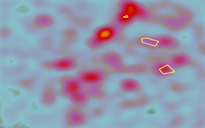
To identify areas with geographic characteristics similar to known coal mining sites, three representative polygons (mine_query, outlined in yellow) were selected as query features. These were run against a raster of pre-computed location embeddings for the full study area using the Find Similar Features Using Embeddings tool.
Rather than relying on hand-picked spectral indices or manually engineered features, this approach uses embeddings that encode the underlying spatial and spectral patterns of each location, capturing texture, context, and structure in a way that’s difficult to replicate with traditional band math alone. The tool computes a similarity score between every pixel’s embedding vector and the embeddings of the query polygons, effectively asking: How close is this location, in feature space, to the areas already known to be mines?
The resulting similarity scores were rendered as a heat map, with the red-to-yellow gradient (sparse to dense) indicating increasing similarity to the query features. To validate the output, high-similarity zones were compared against validation_mines_cils, a reference layer of previously mapped mining locations (black points). The strong spatial correspondence between the model’s top similarity clusters and the validated mine sites confirms that the embeddings captured the distinguishing geographic signature of coal mining activity—not just at the three query sites, but across analogous, previously unlabeled areas in the study region.
Identify Similar Himalayan Mountain Terrain
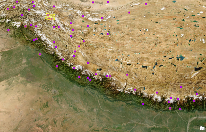
Here, a single polygon located in the high-elevation terrain of the Himalayan range (Query_feature_Himalaya, yellow) was used as the query feature, run against a candidate set of location embeddings spanning the broader Himalaya–Gangetic transect.
The tool returned the output embeddings feature class (purple points) as the candidate locations with the closest embedding vectors in feature space to the query polygon. As expected, the returned matches align closely with the high-relief, snow-covered mountainous terrain running along the Himalayan arc, while candidate points in the flat, cultivated lowlands to the south were not selected. This confirms that the embeddings encoded terrain-level characteristics such as elevation, ruggedness, and land cover typical of high mountain environments, allowing a single representative sample to generalize across an entire mountain range without manually defined rules for slope or elevation thresholds.
Identify similar features on the Gangetic plains
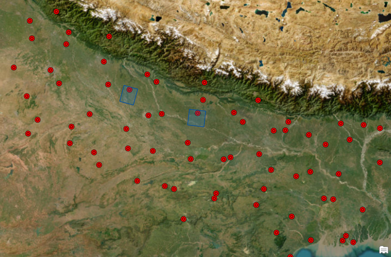
In this case, two query polygons (Query Features, blue ) were selected from the flat, agriculturally dominated Gangetic plains, south of the Himalayan foothills. These were compared against a broader set of embedding candidates distributed across both the plains and the mountains. The threshold to get the similar embeddings is set to 0.5.
The resulting output embeddings feature class (red points) shows a clear concentration within the plains region, closely tracking the low-lying, densely cultivated and settled landscape characteristic of the Ganges basin, while candidate points in the Himalayan terrain were largely excluded. The embeddings here pick up on the flat topography, land use, and river-plain characteristics that define the Gangetic landscape, again showing that a small number of representative query samples is enough for the model to generalize the target land-cover pattern across a large, geographically diverse study area.
Search for global desert similarity
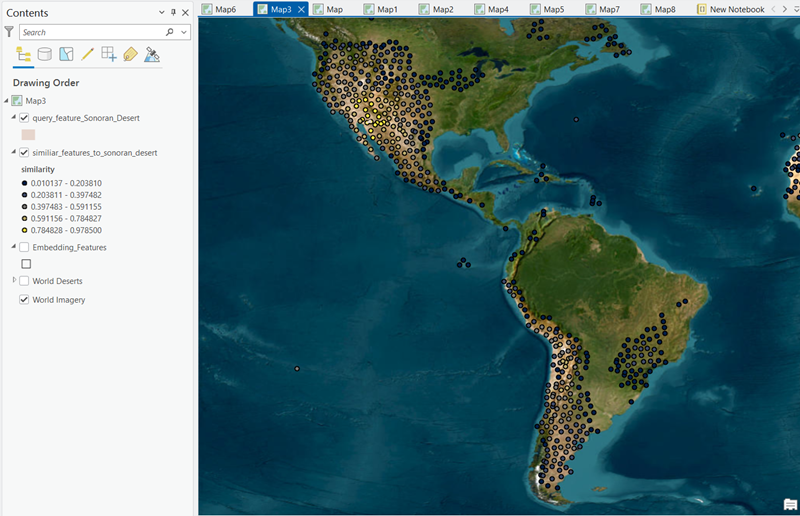
This is a regional close-up of the global desert similarity search shown earlier, focused on North and South America. The similiar_features_to_sonoran_desert layer uses graduated point symbology across five similarity bins, from low similarity (dark, 0.01–0.20) to high similarity (bright yellow, 0.78–0.98).
The highest-similarity points (yellow) cluster tightly around the southwestern United States and northern Mexico, precisely the Sonoran Desert region the query feature was drawn from, confirming the model correctly recognizes the query’s own surrounding landscape as most similar to itself. Moving outward, scores fade through orange and brown as the terrain transitions into the Rockies, the Great Plains, and the more humid eastern US and Central America, dropping further (dark points) across the tropical Amazon basin.
Notably, the model performs just as well at picking out arid terrain much farther south: elevated similarity points appear along the Atacama Desert on the Peru–Chile coast and the Patagonian steppe in Argentina, which are both true desert and semi-arid environments, despite being on a different continent from the query feature and separated from it by the Amazon rainforest. This confirms the model is responding to genuine environmental similarity (aridity, sparse vegetation, and surface reflectance) rather than simple geographic proximity to the query point, which is the same behavior that drove the strong global clustering seen in Figure 4, now visible at a finer regional resolution within a single continent-pair view.
3. Clustering
While the previous examples used embeddings for weakly supervised similarity searches, comparing candidate locations against known query feature embeddings can also be used unsupervised, displaying the data’s default groupings.
The workflow starts with the Generate Embeddings Using AI Models tool, which produces a location embedding vector for each feature in the study area, encoding its underlying spatial and spectral characteristics. These embeddings are then passed through Extract Embedding to Fields,which unpacks each vector into individual numeric attribute fields, converting the embedding into a standard multivariate table that the ArcGIS Pro statistical tools can work with directly.
With the embedding dimensions now available as fields, they’re used as input in the Multivariate Clustering tool, which groups features based on statistical similarity across all embedding dimensions simultaneously with no predefined query feature and no training example required. The tool can detect the optimal number of clusters automatically, or the analyst can specify it directly, depending on how much control is needed over the resulting classification.
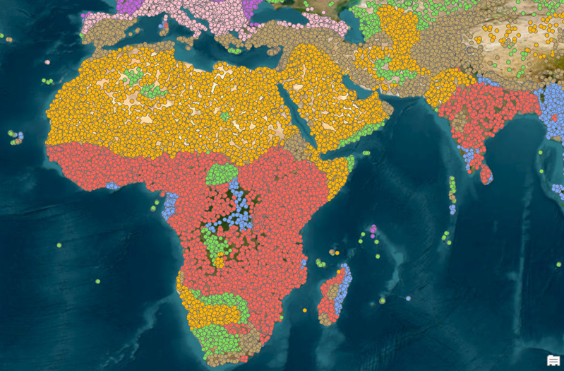
The result, shown in Figure 5, is a set of distinct clusters—7 in above example—each rendered in a different color that emerge directly from the structure of the embedding space. The pattern shows the clusters align closely with recognizable large-scale landscape types rather than administrative or political boundaries. The orange cluster traces the Sahara and Arabian deserts almost precisely. Red highlights the humid tropical belt across Central and West Africa. Green marks vegetated transition zones and highlands, while blue is seen around the Congo Basin’s dense equatorial forest core. Even without a labeled example, the embeddings alone are enough to separate desert, savanna, tropical forest, and montane environments into coherent, spatially contiguous groups.
This makes for a useful complement to the similarity-search workflow shown earlier. The Find Similar Features Using Embeddings tool answers “Where else looks like this place I already know?”, but running the Multivariate Clustering tool on the same embeddings answers a broader question, “How many distinct landscape types exist in this study area, and where are their boundaries?” Used together, the two tools provide both a targeted search capability and a way to discover landscape typologies that analysts may not have anticipated, all built on the same underlying embedding features.
4. Train a predictive model
Beyond similarity search and clustering, location embeddings can also be used to train or improve machine learning models for regression and classification tasks. The Train Using AutoML GeoAI tool includes a Use Location Embeddings option that automatically enriches your input dataset on the fly with location embeddings before training, without requiring a separate embedding generation step. This is particularly valuable for datasets in which the target variable has a strong but hard-to-quantify spatial dependency—such as forest density, population distribution, health outcomes, or groundwater condition—where nearby geographic context often carries as much of a predictive signal as the tabular attributes themselves.
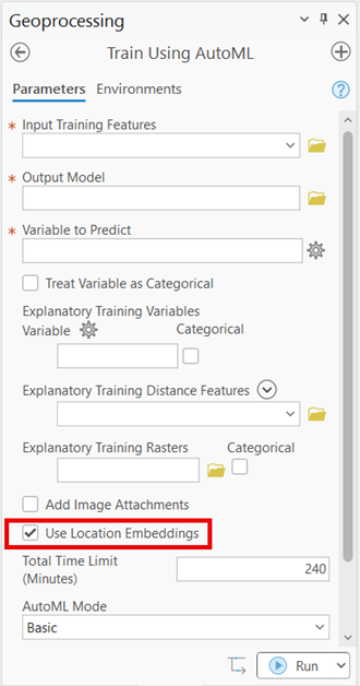
When this option is enabled, Train Using AutoML generates location embeddings for each training sample. This process is described in more detail in section 1.f of the AutoML training workflow, See How AutoML Works to learn more about the underlying process. View a sample notebook demonstrating location embeddings for enhanced house price prediction in King County using AutoML for a worked example.
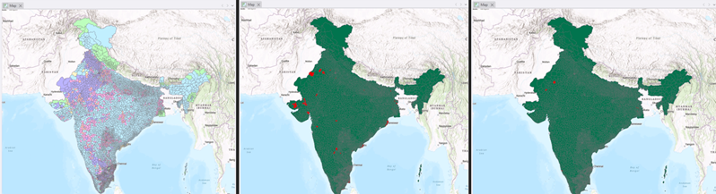
In this case, administrative block boundaries across India (as shown in the first image of Figure 7) were symbolized by groundwater class — Critical, Safe, Saline, Semi-Critical, and Over-Exploited — serving as the input geography and ground-truth reference for the classification task. Two AutoML models were then trained on this data: one without location embeddings, and one with the Use Location Embeddings option enabled as show in Figure 6.
The baseline model, trained without location embeddings, misclassified administrative blocks concentrated notably along parts of western and central India, totaling 112 misclassified areas (red shown in the center image of Figure 7). The model trained with location embeddings enabled, by contrast, brought this number down sharply to just 30 misclassified blocks, with the vast majority of the country now correctly classified (green shown in the third image of Figure 7). This reduction underscores the importance of location embeddings in spatial groundwater classification . Neighboring blocks tend to share hydrogeological conditions, and location embeddings refine the model with spatial context, rather than recording each block as an isolated observation.
Limitations
The following are limitations of the model:
- Temporal coverage—The model is trained on satellite imagery collected between 2022 and 2024. As a result, the learned representations primarily reflect geographic and environmental conditions observed during this period and may not capture significant changes occurring outside this timeframe.
- Limited seasonal representation—Although the training data spans multiple years, it does not comprehensively capture seasonal variations across all regions. Consequently, the embeddings may be less effective for applications in which seasonality plays a significant role.
- Land-only coverage—The model is trained using land-based geographic coordinates. It is therefore expected to perform best for locations on the Earth’s land surface and may not generalize well to open oceans or other non-terrestrial regions.
- Training—The current Global Location Encoder (Sentinel-2) is trained on Sentinel-2 imagery, so embeddings are derived only from its 12 spectral bands. Characteristics outside this scope won’t be represented in the embeddings.
- Limited interpretability—As with most deep-learning-derived representations, individual embedding dimensions don’t correspond to directly interpretable physical variables. This can make it harder to explain why two locations were scored as similar or grouped into the same cluster, beyond pointing to the overall pattern.
Conclusion
Location embeddings offer a new lens for GIS, turning raw coordinates into more accurate representations of place that require minimal training data, do not require manual feature engineering, and can be used in a variety of scenarios, from study-area mineral exploration to regional terrain mapping to global desert detection.
References
- For a full overview of the embeddings-based analysis toolset in ArcGIS Pro, see An overview of the Embeddings Based Analysis toolset.
- To download or explore the Global Location Encoder model item, visit the ArcGIS Living Atlas item page.
- Introduction to the embeddings
- Concepts of the embeddings
- Use the embeddings



Article Discussion: