Imagine you’re in Ottawa, Canada and you need to get your hair done ahead of the wedding you’re in town for. There are two salons you’re considering, but one salon is further away from where you’re staying. That’s an easy call, right? You go to the salon that’s closer. But hang on, there’s a differentiating factor between the two locations: one salon carries a wide variety of hair products, and the other only carries one brand. And huh, the one with the fabulous, wide selection of products is the location that’s further away. Will the attractiveness of the fabulous salon outweigh the shriveling effect that distance has on your desire to go there?
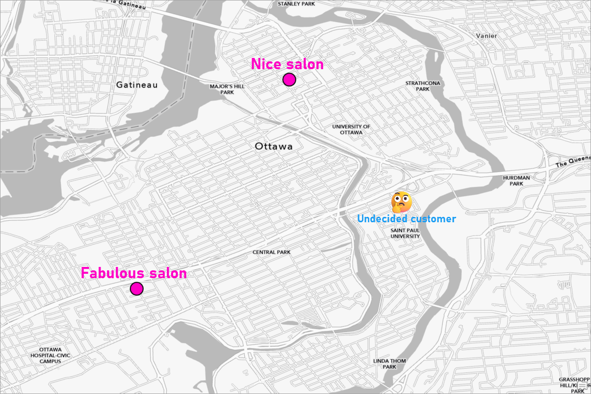
Consumers face these types of decisions every day, presenting a thorny problem for business owners. How can you create accurate trade areas that account for that “x factor” that draws customers in spite of greater distance?
Equal probability trade areas
The Generate Huff Equal Probability Trade Areas tool in ArcGIS Business Analyst Pro allows you to create trade areas that go beyond distance alone in mapping the regional dominance of competing locations. You can effectively weight locations based on attractiveness, whether you define that as the number of parking spots, average customer review, or brand assortment. As long as there is a numeric attractiveness variable in your input data, you can use the tool, and even modulate the strength of that attraction using variable exponents.
You’ll find the tool in the Business Analyst toolbox, within the Trade Areas toolset.
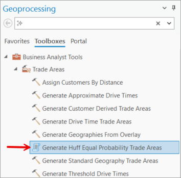
You can use Huff equal probability trade areas to map the push and pull of attractiveness versus distance for your stores. Trade areas will be drawn based on two crucial fields: Distance Exponent and Attractiveness Variable & Exponent.
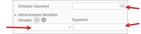
You’ll use these parameters to specify how much distance and attractiveness shape your trade areas. It’s push and pull: Distance is a negative exponent potentially pushing people away, while attractiveness variables carry positive exponents and draw people in. The tool’s calculations treat more attractive locations as having more gravity—essentially, a location with larger attractiveness becomes “closer” than plain Euclidean distance implies.
The fabulous salon example
Using the fabulous and less-fabulous Ottawa salons as an example, let’s say you own the two salons and want an idea of the trade areas around your locations. If each store’s influence were just based on a customer’s distance to the salon, the trade areas might look like this:
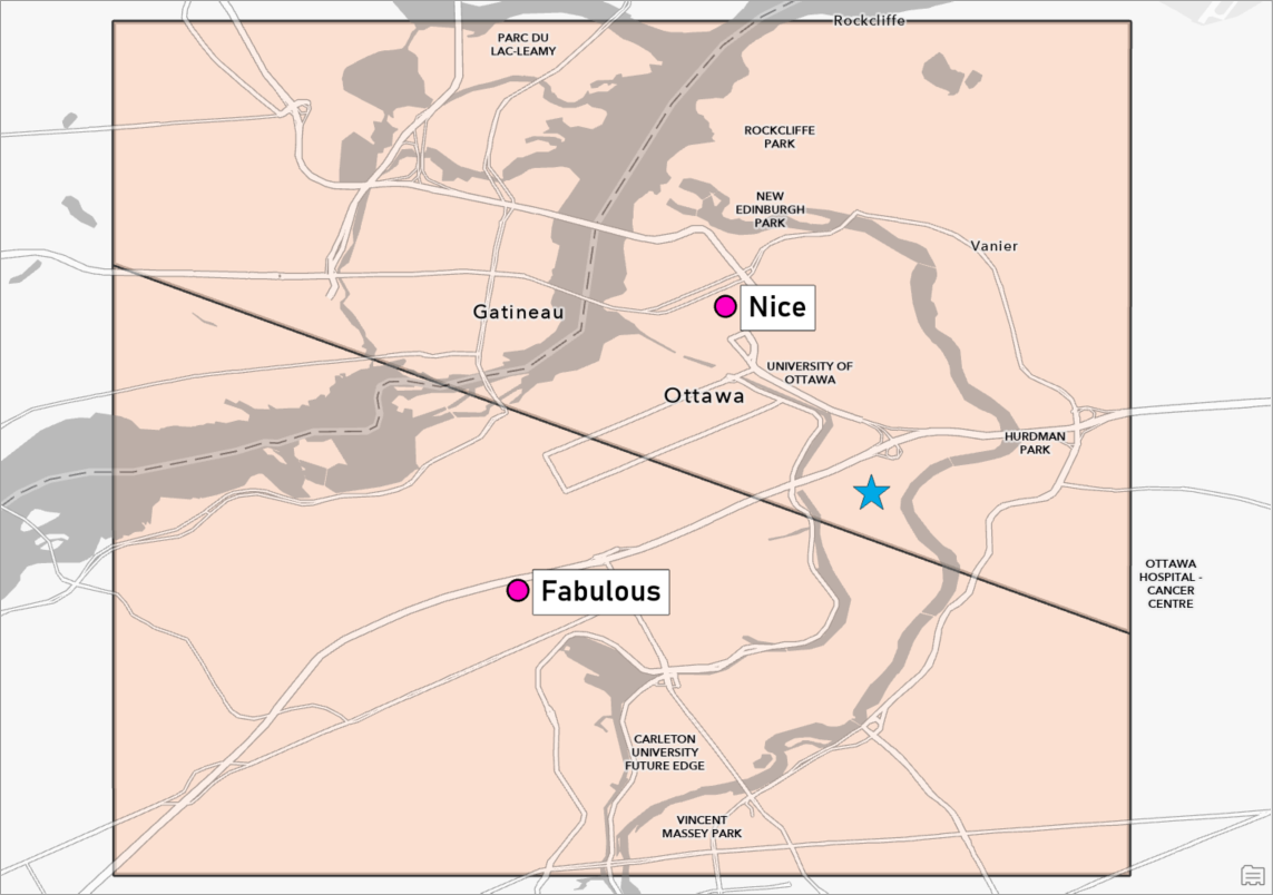
Without attractiveness factored in, a line is drawn halfway between the locations and all customers just go to the salon nearest to them. But if we use the numeric data contained in the salons layer, we can pick an attractiveness variable that will draw smarter trade areas.
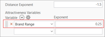
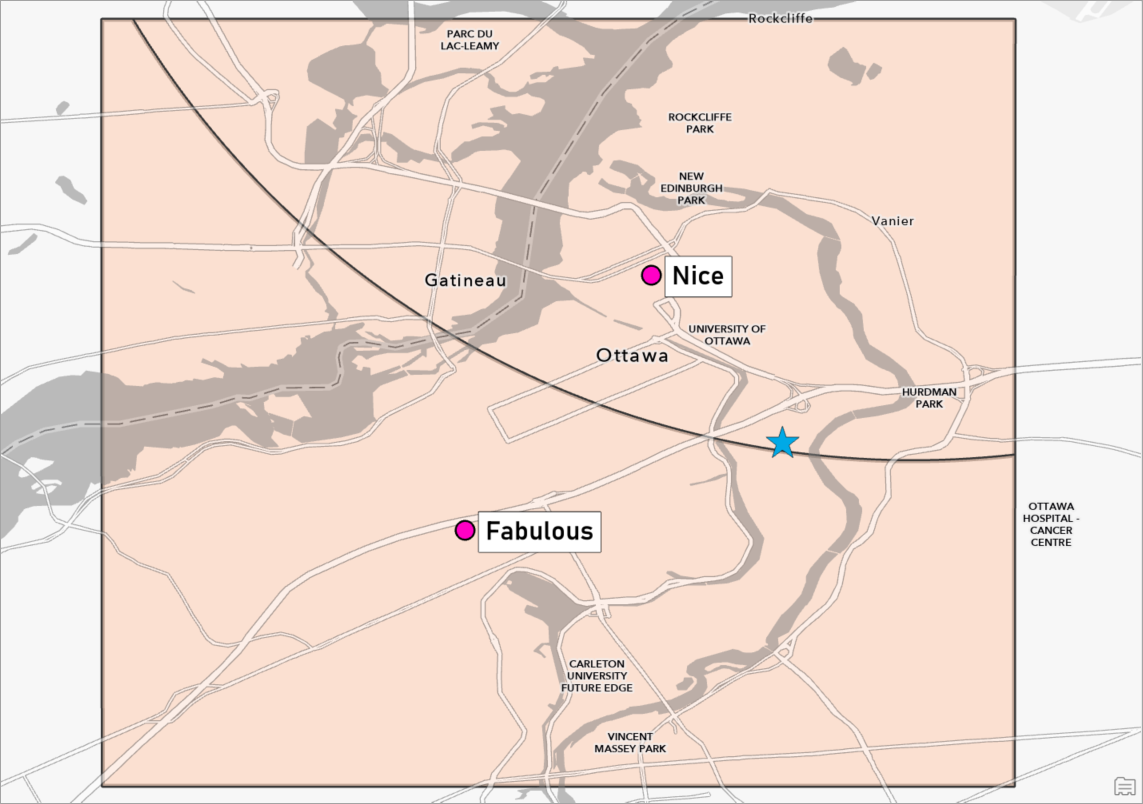
In this case, we’ll use the product selection (brand range) to quantify the attractiveness of each location. Let’s set the attractiveness exponent at 0.25, representing a real but slight pull based on the brand range. (To read more about how to choose an exponent, see Suggested exponents.)
This pull starts to curve the boundary between the trade areas; you can see that our undecided customer is now at the very edge of the dominance zone for the nice salon.
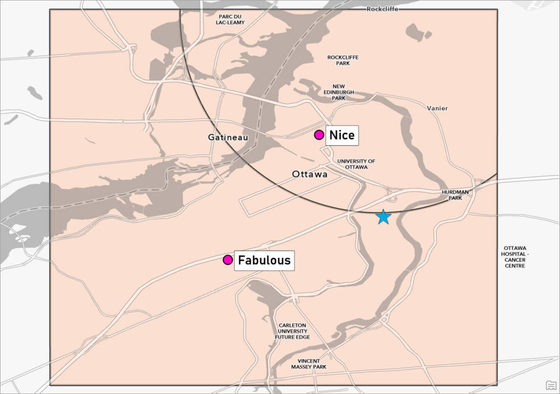
Let’s say we discover that the range of brands is actually more influential on our customers than we thought. We adjust the exponent to reflect this discovery. With the attractiveness exponent at 0.5, the undecided customer is now on the other side of the border:
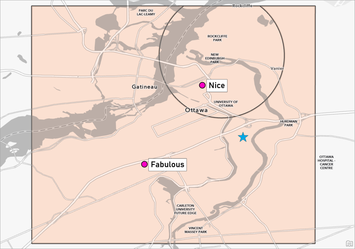
As we keep notching up the strength of the attraction to a large range of brands, the trade area for the fabulous salon gets larger and larger. At a 0.75 attractiveness exponent, the customer is firmly within the bounds of the further-away salon.
Who decides what’s attractive? You.
Of course, not every business or even every salon uses brand range as a way of denoting attractiveness. None of this is set in stone—the tool empowers the user to define the term for their own industry and use case. The possibilities for different industries and attractiveness factors are limitless:
- Retail or service businesses might use number of employees to approximate store capacity or service level
- Brick-and-mortar stores might use the number of parking spaces as a proxy for attractiveness
- Urban businesses might use a transit accessibility rating to assess their different locations
Fascinatingly, if we return to the salons but use a different variable for attractiveness, the outlook changes completely. If we select Average Customer Review as the measurement of attractiveness, suddenly the fabulous location is looking a little less “fabulous”:
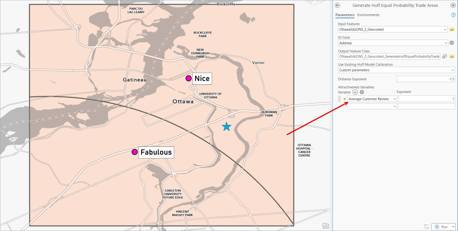
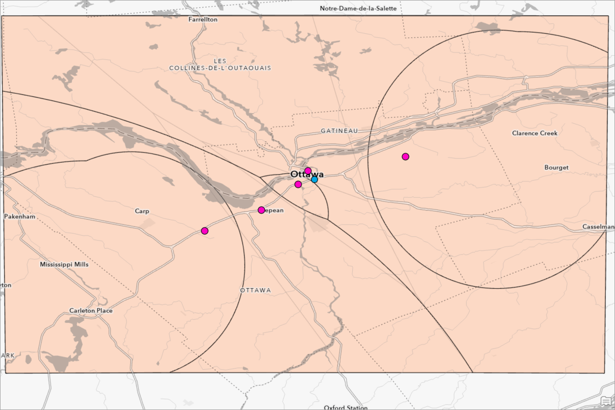
Furthermore, trade areas for more locations look super interesting. Here are the trade areas for five locations of this salon franchise in Ottawa, weighted by average customer review:
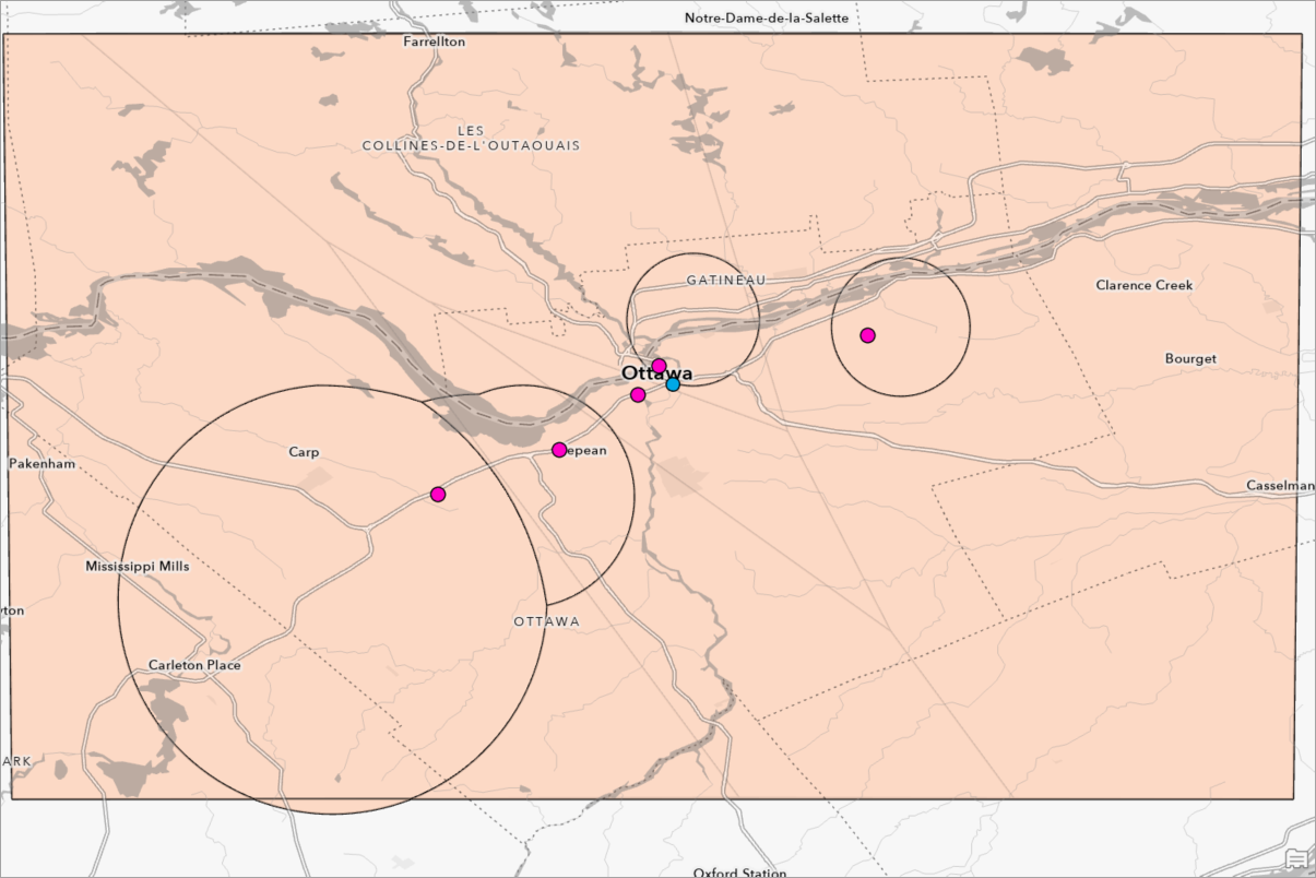
And here are the same five salons weighted by brand range (the “fabulous” location dominates):
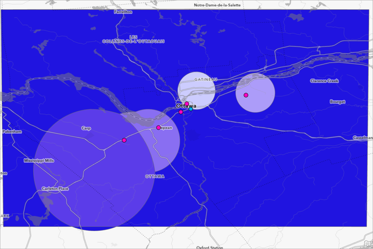
You’ll notice, too, that you can use multiple attractiveness factors in the tool, which means you can decide which factors are the most important, and how important they are for attracting customers. Feel free to have a blast styling these trade areas based on size as well!
The possibilities and use cases are endless. Happy Huff-ing!
This article uses ArcGIS Business Analyst Pro 3.8. The Ottawa Salons feature layer was adapted from the data in the Get started with ArcGIS for Excel tutorial.
Resources
To continue your Business Analyst journey, visit the following resources:
- Business Analyst product overview page
- Review pricing and purchase Business Analyst
- Business Analyst resources page
- LinkedIn user group
- Business Analyst Web App video channel
- Business Analyst Pro video channel
- Business Analyst on Esri Community
- Business Analyst Web App login page
- Email the team: businessanalyst@esri.com


Article Discussion: