Isochrones, drive time polygons delineating the area around a location, are a particularly common method of determining the area used for assigning demographic attributes to a location for modeling and forecasting. Even when creating isochrones for stores of a single brand, all stores are not created equal. One single value cannot be used for all stores because peoples’ willingness to travel varies. Although using customer data is preferable, in the absence of customer data, a combination of available enriched data variables and Arcade scripting can be used to create uniquely sized isochrones for every location.
Earlier this year my colleague Kyle wrote an article about using Arcade expressions with Business Analyst. This article expands on this concept, this time using demographic data to determine the correct isochrone size for each respective location using a metric of customers’ willingness to travel. Frequently this comes from the customers’ home locations and preferred stores based on a loyalty card or even from human movement (cellphone tracking) data purchased from a data provider. In the absence of either of these, it is possible to use an indication of willingness to drive, average commute time, as a proxy to create isochrones around stores. This is what we are going to cover here.
This value, average commute time, is not included as a single value in Esri’s demographic data. However, the number of people who commute within ranges of time is available. To create isochrones for forecasting we need a single value. This single value can be derived from the available data using a little Arcade scripting as a parameter in the Generate Drive Time Trade Areas geoprocessing tool. First, we need to get the data to start with using enrichment.
Enrich Locations
Since we do not have any customer data to work with, we need a value for how much potential customers are willing to travel to each store location. Enrichment adds factors or attributes with a geographic area, but we have points. Fortunately, the Enrich Layer (Business Analyst toolbox) tool includes the ability to specify how to sample the geographic area surrounding an input point.

First, we need to select variables representative of customers’ willingness to travel to a location. As we discussed earlier, we can use commute times as a decent indicator. When searching for commute in the enrich variables. There is no single average commute time, but there are variables with the count of people based on commute time ranges.
- Commute to Work: <5 min
- Commute to Work: 5-9 min
- Commute to Work: 10-14 min
- Commute to Work: 15-19 min
- Commute to Work: 20-24 min
- Commute to Work: 25-29 min
- Commute to Work: 30-34 min
- Commute to Work: 35-39 min
- Commute to Work: 40-44 min
- Commute to Work: 45-59 min
- Commute to Work: 60-89 min
- Commute to Work: 90+ min

Next, the default option for enriching points is creating a one-kilometer straight-line buffer around the point used for apportioning attributes. However, the Enrich Layer tool allows us to select a lot more options. In our case, to better represent the area surrounding each of our locations for enrichment, we are going to use a 12-minute drive time polygon to sample around each point for enrichment.
Also, if you are astute, you will notice in the screenshot we are also using Rural Driving Time. The difference between Driving Time and Rural Driving Time is whether gravel roads are avoided. Since solving for a farm supply in rural areas, we are using Rural Driving Time.
Now, with the data enriched, we need to create the isochrones around each store, but we also need a single value for each location. Currently, we have 12 values, and they are counts, not average drive times. Fortunately, we have math.
Make the Machine Do the Work
The process of calculating this value is incredibly tedious and error-prone to do manually. Fortunately, we can script the calculation of this value using Arcade right in the input for the Create Drive Time Trade Area geoprocessing tool.
Create Drive Time Trade Areas

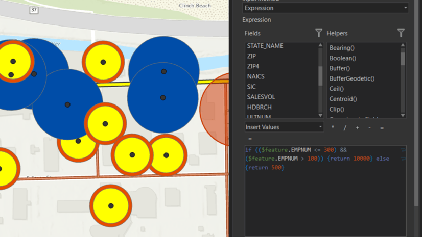
This is where the magic happens, where we make the computer do the work…always a good thing. Above we discussed how average is the sum (total commute time) divided by the count (all people commuting). We can use Arcade to calculate these values right in the Generate Drive Time Trade Areas tool. Although most of it is visible in the image, you can also take a look at it as a Gist.
Just as discussed earlier, not only are we getting the average per location, but we also are dividing this by two – using half of the average to create an isochrone for each farm supply location. Once complete, we have isochrones, drive time polygons, for all our farm supply locations based on the commuting habits in the surrounding area. All it requires, after we have store locations to work with, is two steps, Enrich Layer to get the commute drive times, and Generate Drive Time Trade Areas to create the isochrones…with the help of math and a little Arcade scripting.
Create Drive Times Using Arcade
Once complete, as is evident in the map toward the top of this article, no two drive times are the same, and due to the inherent geographic barriers in Wisconsin, all the lakes and rivers, the size and shape of the polygons varies widely…with obvious implications for how many potential customers are encompassed in each isochrone. From here, these new geographic areas are ready to be enriched with demographics to fuel performance forecasting models.


Article Discussion: