Connecting locations with optimal paths

This is the fourth in a four-blog series discussing Distance Analysis. In the first blog, we demystified distance analysis. In it, we identified the three major aspects for performing distance analysis, 1) calculate the straight-line distance, 2) determine the rate the distance is experienced by the traveler, and 3) connect identified locations with optimal paths.

The second blog focused on the first aspect, calculating the adjusted straight-line distance while incorporating barriers and the surface distance.

The third blog covered the second aspect, determine the rate the adjusted straight-line distance is experienced by the traveler. We altered the adjusted straight-line distance accounting for the cost surface, vertical and horizontal factors, and source characteristics to create the accumulative cost-distance raster.

For certain applications, identifying the least-cost distance is the end product, such as an input criterion in a suitability model. But many times, we want to identify the optimal paths for the traveler to efficiently move between locations.

The two main approaches to create optimal paths are:

1. Connect specific locations to one another
2. Create an optimal network of paths to move effectively between a series of regions

We will begin with the first approach, connect a specific location to another known location.

To do so, a general two-step process is used:

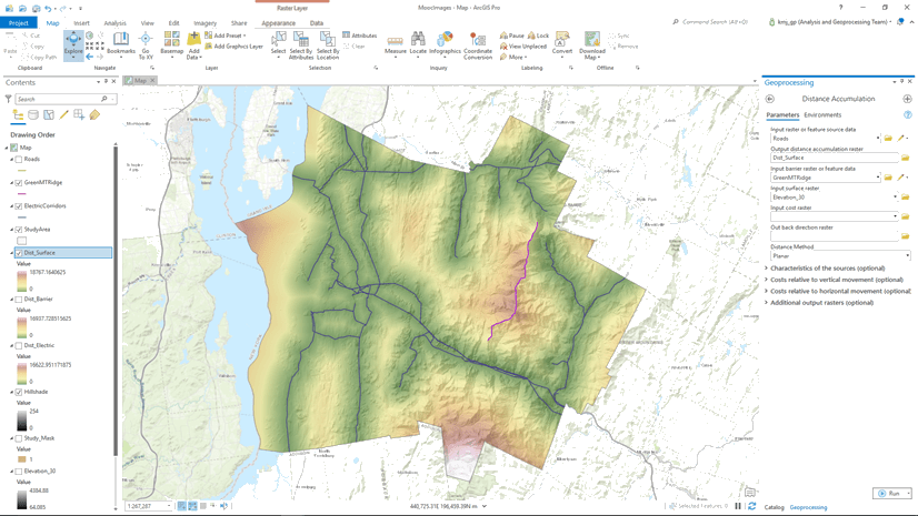
1. Run Distance Accumulation (or Distance Allocation) to create the accumulative cost-distance raster. For each cell in the raster, the shortest or least-cost distance is calculated from the closest or cheapest source.
2. Run one of the Optimal Path tools (Optimal Path As Line or Optimal Path As Raster) with the output rasters from Distance Accumulation (the accumulative cost and back-direction rasters), as well as the destination as the input.

To understand these two steps, let’s recap where are we at in the blog series. In the second and third blogs we focused on calculating the accumulative distance using the Distance Accumulation tool (step 1 above). In the resulting accumulative cost-distance raster, what we know is, for each cell, the least-cost to reach each cell from the closest or cheapest source accounting for the surface distance and barriers and the rate that distance is experienced adjusting for the cost surface, vertical and horizontal factors, and the source characteristics.

To identify optimal paths, we need to know the way to travel through the cells to reach the location that produces the least cost. What we need to know is the least-costly path to reach a cell.

Distance Accumulation not only outputs a raster identifying the least-accumulative cost to reach a cell, it also outputs an optional back-direction raster. In the back-direction raster, for each cell, the direction that should be taken from the cell in route on the least-cost path to a cell is identified.

In the new algorithms mentioned in the third blog, planes are fit to produce the precise route to move through a cell. To capture this realism, the values assigned each cell in the back-direction raster are continuous compass values ranging from 0 to 360 degrees. The directions are not the 1 to 8 values that were used to identify which cell center to move to as was done in the cost distance legacy tools.

The destination you want to travel to, and the output accumulation and back direction rasters are the input to the Optimal Path tools. An Optimal Path tool creates the optimal path by following the directions assigned each cell in the back-direction raster back to the source.

What is particularly exciting is, as mentioned above, the path is not a simple trace through cell centers. The Optimal Path tools connect where the path enters the cell by looking at the directions assigned to the cell itself and the neighboring cells and determines how to most effectively pass through the cell. Generally, the path does not pass through the cell center but passes through the cell irrespective of the cell structure. As a result, you can move through, say, just a corner of the cell. The result is a realistic portrayal of how the traveler will move through the landscape.

In this first scenario for creating optimal paths, we knew which location needed to be connected to another location. This can be used to:

1. Site an electric line to run between two known substations
2. Route the least-costly road to connect to a new school
3. Determine the shortest water distance between two ports

For additional information see Connect locations with optimal paths.

But for certain applications you may have a series of locations (which we will refer to as regions) and you want to move between them in the most efficient way possible. Applications include:

1. Connecting a series of wildlife patches with movement corridors
2. Creating a series of logging roads to efficiently extract timber
3. Produce a hiking trail network for fire fighters to travel between headquarters

Here we want to create a network of paths that connect all the regions. But how do we determine which region should be connected to which? All of them to each other? Connect the ones that are closest to one another?

To connect each region to all the other regions would produce too many paths especially when there are many regions. Also, since the paths would be created independent of one another, there will be a lot of redundancy.

To connect the regions that are closest is done in many applications. The problem with this approach is that two regions maybe close in distance but maybe far in cost. For example, a mountain or major river maybe between two regions. The regions might be close in proximity, but the mountain or river makes them far in cost.

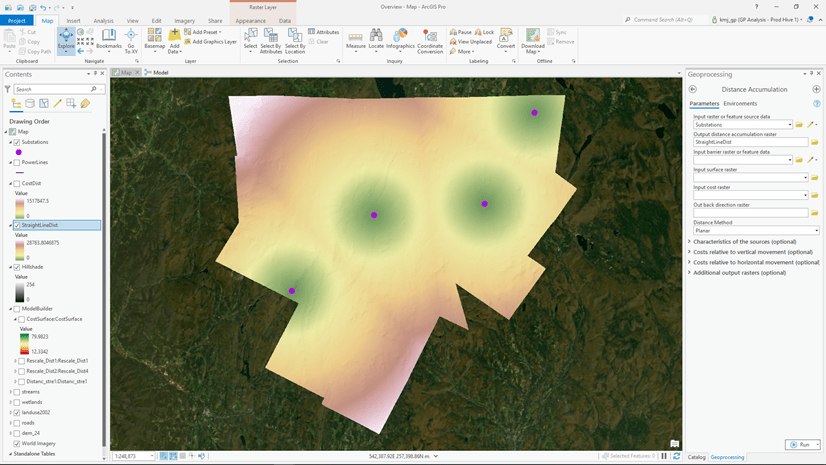
This leads us to the solution used in Optimal Region Connections. The tool connects the regions that are closest based on cost. Let’s see how the tool conceptually works.

1. Identifies which regions are cost neighbors.
2. Connects the regions with the least-cost paths.

3. Converts the resulting paths into a graph. The input regions are the nodes, the paths are the edges, and the total accumulative cost for each path are the weights on the edges.

4. Solves the Minimum Spanning Tree (MST) using graph theory. The MST identifies the network of edges (paths) that connects all the nodes (regions) in the most cost-effective manner.

5. Maps the resulting MST back to Pro to create the final optimal-path network.

In the resulting network, the traveler can reach any region (sometimes moving through another region to reach a distant region) the most efficient way possible. The optional network of paths to each of the cost neighbors is also a commonly used network.

For additional information see Connect regions with the optimal network.

When creating the MST, the direction of the traveler is irrelevant. If directionality matters, you must use the first two-step approach identified above, the Distance Accumulation/Optimal Path tools.

Thus far, we have connected specific locations with an optimal path, and we connected a series of regions with the least-cost network. But the resulting paths are lines and sometimes the traveler needs to move through a wider path than just a line, they need to move through a corridor. Applications include:

1. Connecting two patches of bobcat habitat with a wildlife corridor
2. Identifying the corridor that a proposed electric line must stay within

Why do we not just take the above paths and buffer them? With a buffer, you may include highly undesirable locations such as a factory in a wildlife corridor. Instead the path can be expanded by a specified maximum accumulative cost to create the corridor. Euclidean or straight-line buffer is an objective distance. A corridor based on cost captures how the subject interprets the world and then makes decisions.

Think of a corridor as containing all possible paths between the two regions that are below the specified cost threshold. That is, as long as you move within the corridor, you are on an optimal path that is below the cost threshold.

To create a corridor the Distance Accumulation and Corridor tools are used. For additional information see Connect locations with corridors.

In summary, distance analysis can be simplified into an integrated story:

1. Calculate the straight-line or Euclidean distance.
2. Adjust the straight-line distance with the surface distance and barriers to identify the actual shortest distance a traveler would take between two points.
3. To understand what the traveler experiences, determine the rate that adjusted distance is encountered by applying a cost surface, vertical and horizontal factors, and the source characteristics to create an accumulative cost-distance raster.
4. Connect locations optimally over the accumulative cost-distance raster by connecting specific locations with the optimal path, connecting a series of regions with an optimal network, or connecting locations with a corridor.

Distance analysis is about adjusting the distance it takes to move across each cell to capture the interactions and decisions of the traveler as they move through their environment. However, please do not lose sight in the details, it is all just distance.