This is the third in a four-blog series discussing Distance Analysis. In the first blog, we demystified distance analysis. In it, we identified the three major aspects for performing distance analysis, 1) calculate the straight-line distance, 2) determine the rate the distance is experienced by the traveler to create a distance accumulation raster, and 3) connect identified locations with optimal paths over the accumulation raster.
The second blog focused on the first aspect, calculating the adjusted straight-line distance while adjusting for barriers and the surface distance.
This blog will focus on the second aspect, determine the rate at which the adjusted straight-line distance is experienced by the traveler. Here we will simulate how the traveler moves through the landscape, capturing the decisions and choices they make. This is one of my favorite parts of distance analysis. Capturing the traveler’s experience, to me, is the primary goal of many problems.
When calculating the shortest distance between two points it is assumed the traveler is a bird or an airplane and they are ignoring the environment they are flying through.
To account for what the traveler is experiencing, you must think as if you are the traveler. Imagine you are on foot and traveling between two locations. What would you consider in order to move in the most efficient way? The first question you may be asking, how do you define efficient? Is it in the shortest time? The least amount of energy expended? Or the route in which you see the best views? As you might expect, your goal will dictate the decisions you make as you travel through the landscape.
Let’s say you want to move between the two points in the shortest amount of time. What would influence your decisions to do so? As mentioned in the first blog, there are four factors that affect how you encounter the distance.
Obviously, what you are traveling through will dictate how fast you can move. For example, you can move faster through certain land use types such as fields and open areas than if moving through a swamp. In our case, time is our cost and each cell will be assigned the time per unit of distance to move through each cell producing a cost surface. For additional information see Adjust the encountered distance using a cost surface.

Second, if you are moving uphill, downhill, or across the slope in a cell will influence your speed. You will walk at a slower rate going uphill than traveling on a flat surface, therefore it will take longer. How you encounter the slope as you move through the cell influences the time or cost to move through the cell. This extra time or effort is referred to the vertical factor. For additional information see Adjust the encountered distance using a vertical factor.

Third, if you are heading into a strong wind you will move slower. This would be more evident if you are on a bicycle, you will be able to cover the distance units at a faster rate with the wind at your back. For additional information see Adjust the encountered distance using a horizontal factor.

Well, that brings up the fourth factor influencing the rate you cover the distance units, the mode of travel. If you are on an All-Terrain Vehicle versus foot you will be able to cover the distance units at a faster rate. You can control the mode of travel through a multiplier using the source characteristics. For additional information see Adjust the encountered distance using source characteristics.

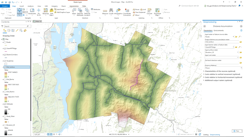
To determine the least-accumulative cost from a source to each location in the study area accounting for the cost surface, vertical and horizontal factors, and source characteristics discussed above, the calculations are broken into many individual decisions based on moving through each cell.
First, the adjusted distance for each cell from the closest source is identified accounting for the surface distance and barriers if specified (the first aspect for distance analysis identified above).
Then, for each cell, the rate the adjusted distance is covered by the traveler is determined. As identified above, there are 4 possible rate adjustments:
- if a cost surface is specified, the adjusted distance is multiplied by the cost to move through the cell.
- if a vertical factor is specified, how the traveler encounters the slope is identified. A vertical cost factor is determined identifying the extra cost to overcome the slope (higher cost equals a higher factor), and the distance is multiplied by that factor.
- if a horizontal factor is specified, the way the traveler encounters a horizontal factor such as wind is identified. A horizontal cost factor is determined, and the distance is multiplied by the factor.
- if the characteristic of the mover is identified such as a multiplier is specified (capturing the mode of travel), that multiplier is applied to the adjusted distance.
The results of the four rate adjustments determines the cost to move through a cell. The total cost (the sum of the individual calculations) to reach a cell is added to that cell’s cost to identify the total accumulative cost to reach the cell. Since the four adjustments are rates, they must be in the same units. That is, if the cost surface is based on time, then the vertical and horizontal factors and source characteristics need to be in time. You cannot mix the units of the rates for the different cost factors.
However, the calculations are not that simple. You do not just look around you and move into the cell that you can move through the fastest. Then, enter the next cell that you can move through the fastest while moving around the high cost cells. This series of local decisions together probably will not give you the least-accumulative cost to each cell. That is, you can make a local decision that leads you into a series cells that are very costly or time consuming to move through. Instead, it might be better to initially move into a cell that is a little more costly or time consuming that leads you to a series of cells that you can move through quickly. In the latter case, you make local suboptimal decisions to determine the overall fastest route – the optimal decision.
Think of it as the traveler has a bag and each cell has a specified number of marbles corresponding to the cost to move through the cell. As the traveler moves through a cell, they collect the marbles in the cell and put them into their bag. The goal of the traveler is to move between the two locations collecting the fewest marbles possible. In this way, we are simulating the traveler having knowledge of the area and therefore can make optimal decisions when choosing the least-cost path to each cell.
The above are conceptual descriptions of how the calculations are made. But the algorithms underlying the new distance tools (Distance Accumulation, Distance Allocation, and Optimal Region Connections) are revolutionizing how distance is calculated. No longer are we calculating between cell centers but rather a series of planes are being fit between the cells so the true cheapest calculations to move through the cells are determined. Why am I so excited about the new algorithms? Simple, the same reason I am excited about determining the rate the distance is encountered, you are able to realistically determine how the traveler will move through the landscape. And that is the entire point! For a detail description of the calculations see Distance accumulation algorithm.
Wait. There is one more thing we must consider, the direction the traveler is moving. The shortest distance between point A to point B will be the same if traveling from point B back to point A. This also would be true if only a cost surface is entered. But when the vertical and horizontal rate adjusting factors are added, the direction of travel matters. The vertical factor adjusts the costs based on how the slope is encountered. If you are going up the slope, it may be more costly than moving with or down the slope. As a result, moving from point A to B the traveler encounters the slope in a cell differently than moving from B to A. Therefore, the cost to move through the cell will probably be different. As a result, moving from point A to B will more than likely be different than moving from point B to A.
For the horizontal factor, such as wind, the direction the wind is encountered would also vary based on how you enter the cell.
You can control whether you are moving from or toward a source using the source characteristics.
Thus far we have discussed the rate of cost as being time or an abstract cost. However, there are many different costs addressing various applications including:
- Determining the fastest route for a ship to move between ports
- Building a least costly pipeline
- Identifying the preferred corridors for the wildlife to move through
- Creating a trail system that travels through appealing landscapes while providing beautiful views
- Designing a logging road network to safely move trucks between operations
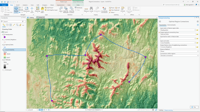
This list leads us into the next blog. Not only do we want to know the least-accumulative cost to reach each location from the closest source, many times we want to identify the optimal path to travel between locations over that least-cost accumulation surface.
As you can see, capturing the rate the distance is encountered can be complex. But do not lose sight, cost distance is only an adjustment to the distance traveled. It is all just distance.

Article Discussion: