A recurring challenge in spatial analysis is the conversion of continuous raster surfaces into vector point features suitable for downstream feature-based workflows. Existing conversion methods either reproduce every cell as a point, producing a dataset that ignores intensity, or aggregate the surface to summary statistics that discard its spatial signature.
The new Raster to Weighted Points tool in ArcGIS Pro is built to address this concern. It converts a continuous raster into a representative point feature class in which point density mirrors surface intensity by preserving the spatial pattern and overall magnitude of the source surface, while producing vector features that slot directly into modeling, enrichment, and operational zone-design workflows.
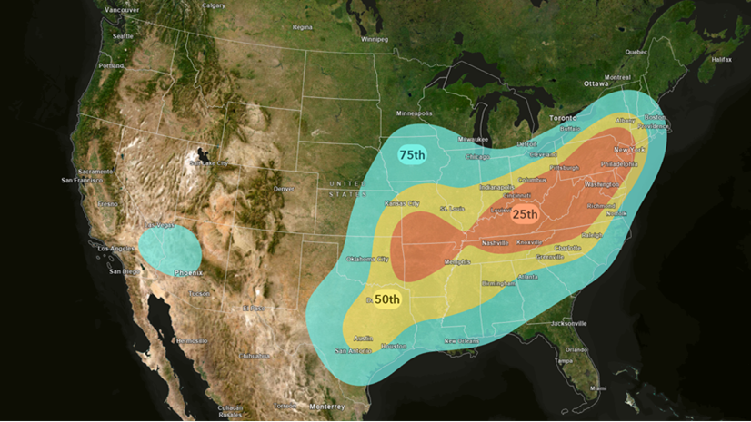
 and the weighted points generated from it (right). Point concentration mirrors damage intensity")
Close the gap between raster surfaces and vector-based analytics
Continuous surfaces are the native output of a large family of spatial analysis functionalities: density and pattern analysis, interpolation, overlay analysis, distance and connectivity analysis, and risk and suitability models. They excel at showing where something is concentrated. But a growing share of analytical workflows—feature engineering, classification, regression, clustering, model validation, uncertainty assessment—assume a tabular structure and often need feature classes as inputs that contain rows of observations, columns of predictors, and a target variable.
Bridging these two worlds has traditionally required compromise. A traditional raster to point conversion will convert every cell into a point, producing files that are bulky and that treat a low-intensity cell the same way as a hotspot. Additionally, the raw input data may not be available, and sharing raw input events can expose personally identifiable information and raise privacy concerns that most projects cannot absorb.
The Raster to Weighted Points tool closes this gap with a simple proposition: generate a specified number of points whose spatial distribution is proportional to the surface itself. Dense areas get more points, sparse areas get fewer, and the resulting feature class behaves like a sample drawn from the underlying intensity.
Use the Raster to Weighted Points tool to model predictive features
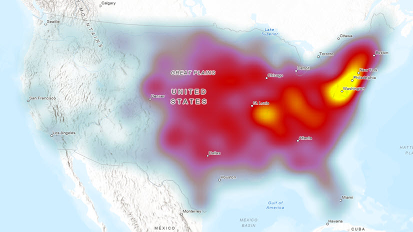
The following example uses a United States flood-risk analytics project to create a kernel density surface from 30 years of flash flood property-damage records between 1996 and 2025. The resulting surface captures where property damage concentrates during flash flood events. The analytical goal is to prepare the input data for a predictive model that relates damage intensity to the property’s elevation, distance to streams, impervious surface cover, and parcel value. The raster alone cannot be used in most downstream modeling workflows.
To run the tool, complete the following steps:
1. Generate representative points.
- In the Raster to Weighted Points tool, set the damage-density raster for Input Surface Raster.
- Set a Maximum Number of Points value (this example uses 50,000) to direct the tool to distribute the points across the study area in proportion to surface intensity.
Damage hotspots along low-lying corridors and drainage outlets attract more points; ridges, uplands, and areas with little or no recorded loss receive correspondingly few.

Because the downstream goal for this example is training a flood-damage regression model and running spatial cross-validation, the Point Distribution Method parameter is set to Fibonacci Lattice. The lattice produces a low-discrepancy, quasi-regular pattern of points within each cell. This distribution minimizes the within-cell clustering artifacts that can bias folded cross-validation and inflate spatial autocorrelation in residuals.
Other distribution methods exist for different analytical purposes. For example, Random is applicable for Monte Carlo workflows, Equal Area Voronoi for uniform representation, and Circular for cartographic clarity. Each produces a visibly different within-cell geometry. See Raster to Weighted Points cfor more details on when each applies.

2. Normalize for modeling
Raw density values are rarely model-ready. Flash flood property-damage losses are famously heavy-tailed where a handful of catastrophic events dominate the distribution while most locations cluster near zero. Feeding that distribution directly into a regression or tree-ensemble model means the few largest values will overshadow everything else and dominate the loss function. Setting Normalization Method to Log compresses the tail, stabilizes variance across the study area, and produces a target variable that behaves sensibly under both linear and nonlinear models.
Other normalization options are available in the tool (for example, Min–Max, Z-Score, Sigmoid, Softmax, or Sum-to-1), and each match a different modeling assumption. The concept documentation covers the mathematical form of each transform and when to reach for it.
3. Enrich and model
The output point layer carries the original cell value, the distributed value if more than one point is generated within one cell, and its normalized counterpart as attributes. These points are ready to be joined with context.
- Use the Extract Multi Values to Points tool to sample elevation, distance to nearest stream, impervious surface percentage, soil hydrologic group, parcel value density, and any other predictor raster at each point location.
The result is a feature class with an attribute table of observations with a target variable and a set of covariates, grounded in the spatial pattern of the original surface.
- Once the attributes are added to the point feature, use the enriched point features in forest-based classification and regression, geographically weighted regression, clustering, and cross-validation.
The points behave like a properly weighted sample of the underlying damage field rather than a raw incident cloud.

4. Design operational zones
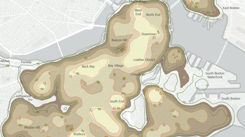
Because point density tracks intensity, the same output doubles as the input to a zone-design workflow. Paired with the Generate Subset Polygons tool, the study area can be carved into polygons that each contain an approximately equal number of points. This means, by construction, an approximately equal share of modeled damage intensity. That is how post-event damage-assessment strata, emergency response and early-warning zones, insurance rating areas, or field-inspection routes are designed when the goal is a balanced workload and equitable coverage rather than equal area.
, translating to roughly equivalent modeled damage intensity per zone")
Why this matters
Three practical benefits carry through the workflow above:
- The spatial pattern survives the conversion—A cluster analysis, a hotspot analysis, or a variogram run on the points recovers the structure of the original raster.
- The output plugs into the rest of the analytical toolkit—Vector point features are the common input in modern spatial data science. So once a surface is represented as weighted points, it can be handed off to Python notebooks, R scripts, dashboards, open-data portals, and GeoAI training pipelines without further translation.
- The points are safe to share—They are representations of surface intensity, not locations of real events or claims, so passing them to partners or publishing them as open data does not reveal individual insurance records, property-level loss amounts, or household identities, which is useful in insurance analytics, public health, emergency management, and any domain in which underlying records are sensitive or regulated.
Bringing surfaces into feature-based workflows
The Raster to Weighted Points tool opens up a new analytical path inside ArcGIS Pro. Continuous surfaces such as kernel density output rasters, suitability rasters, hazard models, accessibility scores can now move directly into the feature-based workflows that drive predictive modeling, sample design, zone construction, and downstream sharing. The flash flood property-damage example captures the pattern, but the same workflow applies anywhere a density or intensity surface needs to become a weighted, model-ready point dataset.
If you are interested in learning more about density tools, see the following conceptual documentation and be on the lookout for future blog articles focusing on Density tools:
- Understand density analysis
- How Kernel Density works
- How Space Time Kernel Density works
- Difference between point, line, and kernel density
Data source
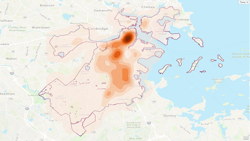
The Crime Incident Reports data used here was collected from Analyze Boston.
References
- Crime Incident Reports (August 2015 – To Date) (Source: New System) – Analyze Boston. (2024). Boston.gov. https://data.boston.gov/dataset/crime-incident-reports-august-2015-to-date-source-new-system

Article Discussion: