USA Geodemographic Embeddings provide a compact numerical representation of thousands of demographic, housing, socioeconomic, and environmental variables. These variables can be used to predict outcomes, but you must determine which parts of the embedding contribute to a prediction. This blog article explores a practical approach to this analysis using the USA Geodemographic Embeddings, AutoML, SHAP, and a food insecurity prediction workflow in ArcGIS Pro.
From input views to interpretable segments
Esri’s Geodemographic Foundation Model (GDFM) encodes four views of geographic context into four 64-dimensional segments, which together represent the 256 dimensions of the USA Geodemographic Embeddings.
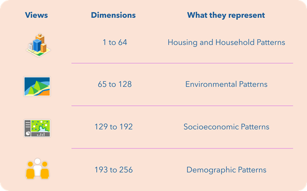
Each segment is a learned representation of its corresponding input view: Housing & Household Characteristics, Environment, American Community Survey, and Age & Race Census, respectively.
These segments highlight the dominant patterns captured in various portions of the embedding. Segment 1 (dimensions 1-64) reflects housing and household patterns, such as occupancy, family structure, and home values. Segment 2 (dimensions 65-128) captures environmental patterns, including climate, air quality, noise, and land cover. Segment 3 (dimensions 129-192) represents socioeconomic patterns related to education, employment, income, and commuting behavior, and Segment 4 (dimensions 193-256) encodes demographic patterns, such as population, age, race, and ethnicity. Together, these segments reveal how the embedding organizes and represents complementary patterns that characterize communities and places.
This structure provides a useful analytical lens for investigating how different aspects of geographic context contribute to downstream models.
A practical example: Predicting food insecurity
To explore embedding interpretability, consider a model that predicts the percentage of people in the United States who were food insecure in 2025, using the County Health Rankings 2025 dataset from ArcGIS Living Atlas.
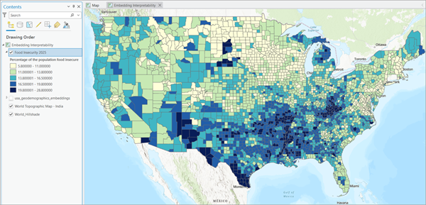
The predictors are the 256 embedding dimensions, and the model is trained using AutoML in Basic Mode, which enables feature importance outputs in ArcGIS Pro.
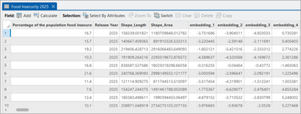
To reproduce this workflow, refer to the Use the embeddings documentation. You must specify a path for the output importance table under Additional Outputs in the AutoML tool pane to get the SHAP importance table. You could also use LightGBM as the algorithm under Advanced Options, which supports SHAP importances among other algorithms supported by AutoML. The How AutoML works documentation provides information relevant in this context.
After training, AutoML produces a SHAP feature importance table containing the importance of each embedding dimension.
SHAP, or SHapley Additive exPlanations, helps explain how features contribute to model predictions. Its global importance values provide a way to identify which dimensions receive the largest average attribution magnitudes in the fitted model across the evaluation samples.
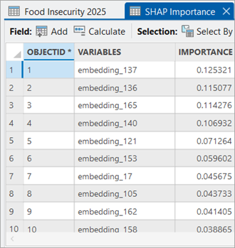
However, by design, the individual dimensions represent learned patterns from the four views used in Esri’s GDFM rather than specific input variables. In this case, SHAP identified embedding_137 (dimension 137) as the most important, but that does not mean you can automatically label it income, employment, or any other original input variable.
To understand the embedding, you must understand how the four embedding segments were mapped to their input views and how they contribute to a specific downstream task.
The key to interpretability: Segment-wise SHAP importance
AutoML’s SHAP importance table output contains the VARIABLES and IMPORTANCE fields. VARIABLES lists the predictor names, which are the embedding dimensions in this example. IMPORTANCE shows the global mean absolute SHAP importance associated with each predictor.
In AutoML, the reported SHAP importance for each embedding dimension is a global mean absolute SHAP value. It summarizes the average magnitude of that dimension’s contribution to model predictions across the evaluation samples. It does not indicate whether the dimension generally increases or decreases the prediction, because the positive and negative SHAP contributions are converted to absolute values.
For a segment, you can calculate its aggregate feature-level SHAP importance by summing the IMPORTANCE values for the embedding dimensions assigned to that segment.
This calculation should be interpreted as an aggregate of feature-level mean absolute SHAP importances. It is not identical to a group-level SHAP calculation based on the signed sum of all SHAP values within a segment. Because positive and negative dimension-level contributions may cancel, the two measures can differ. The segment measure used here represents the total magnitude of the individual dimension-level attributions associated with a segment.
In this case, summing the SHAP IMPORTANCE values for the dimensions 1-64 (Segment 1), 65-128 (Segment 2), 129-192 (Segment 3), and 193-256 (Segment 4) gives the following segment-wise importance table. You can also express them as percentages of total importance.
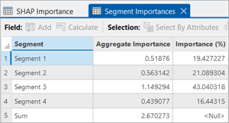
Segment-wise SHAP importance should not be interpreted as the expected decrease in predictive performance if that segment were removed. Measuring incremental predictive value requires a separate analysis, such as retraining the model without the segment or jointly permuting its dimensions and evaluating the resulting performance change.
Read the results: Predicting food insecurity
In this example, Segment 3, associated with the American Community Survey input view, has the largest aggregate mean absolute SHAP importance among the four segments.
This suggests that the fitted model assigns substantial attribution magnitude to patterns encoded from that input view when predicting food insecurity. It does not mean that the model is using a single American Community Survey variable, nor does it imply that the segment has an independent or causal effect on food insecurity.
Similarly, in another use case, if the housing segment accounts for a large share, the model may be drawing heavily on learned housing and household patterns.
These findings provide a descriptive view of how feature-level attribution is distributed across the four learned representations in this fitted model. However, the findings should be interpreted carefully.
Segment-wise SHAP importance does not establish that a particular segment causes food insecurity. Nor does it mean that a specific embedding dimension represents a single variable such as income or employment. Instead, it describes how the model uses learned representations in this predictive task.
From feature importance to contextual understanding
Segment-wise SHAP aggregation provides a bridge between complex latent representations and interpretable geographic themes.
Instead of asking only how much the embeddings help in improving the predictions, you can also ask which broad sources of geographic context the model relies on most when predicting food insecurity.
This approach can be extended to other downstream tasks, including health outcomes, housing markets, socioeconomic indicators, and environmental modeling.
The same embeddings can support different predictive workflows, while SHAP allows you to investigate how the learned representations contribute to each task.
Segment-wise importance is task- and model-dependent. The same embedding segment may receive different importance values for different target variables, datasets, model algorithms, or training configurations. These results should be interpreted as properties of a particular downstream prediction workflow rather than as a universal ranking of the embedding segments.
A more transparent way to use embeddings
Embeddings do not need to be decoded into their original variables to become useful for interpretation.
By combining the documented segment structure of USA Geodemographic Embeddings with SHAP feature importance from AutoML in ArcGIS Pro, analysts gain an additional way to understand how geographic context influences model predictions.
The result is a practical interpretability workflow that uses the 256 embedding dimensions sorted by SHAP feature importance in four segment-level summaries to gain greater insight into model behavior.
As embedding-based GeoAI workflows become more common, approaches like this can help analysts move beyond predictive performance and toward a clearer understanding of how their models use learned representations of geographic context.
Related resources
See the following to learn more:



Article Discussion: