Scientists warn climate change affects many parts of everyday life, including crops needed to sustain humanity. In higher latitudes, warmer temperatures can lead to longer growing seasons and an increase in potential agricultural land, while in other areas, the prolonged higher temperatures may cause a decrease in crop yield. California is famous for its grapes and wines, and I can see acres of vineyards when driving north to Napa Valley. Although grapes can grow in a wide range of climates, the highest-quality wines require a delicate balance of minimum, maximum, and extreme temperatures. To understand whether climate change will affect the quality and quantity of the grapes and wines that make it to consumers, I plan to do some analysis using the multidimensional analysis capabilities in ArcGIS. I’ll be using ArcGIS Notebooks to do my analysis.
Preparing climate data
Growing Degree Days (GDD), a measurement for estimating the growth and development of plants during the growing season, are normally used to predict when a crop will reach maturity. The basic concept is plant development will only occur if the temperature exceeds a minimum threshold, and a plant will only mature if total accumulated heat reaches a certain threshold that is required by the plant.
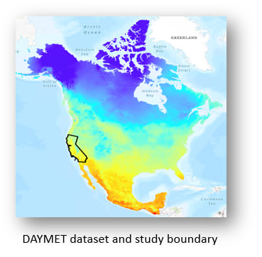
GDD is calculated based on daily minimum and maximum temperatures. The DAYMET dataset contains many climate variables with a temporal resolution and spatial resolution suitable for this study. I downloaded 58 NetCDF files which contain the two variables tmax and tmin—these are the daily minimum and maximum temperatures from 1980 to 2018. To bring this data together, l created a mosaic dataset that references these 58 NetCDF files. Since my study area is California, I used California state boundaries from this service to clip and convert the mosaic dataset to a multidimensional Cloud Raster Format (CRF), which is Esri’s preferred format for storing multidimensional raster data such as this climate data. See this topic for steps on how to create a multidimensional CRF from your scientific data. Now I have the input data that I need.
Analysis workflow outline
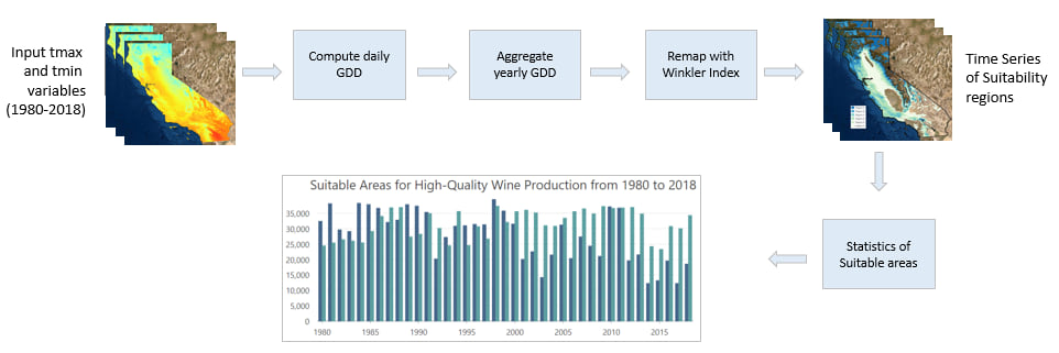
The analysis workflow steps include computing daily GDD from the input temperature variables, aggregating into yearly GDD, classifying the regions using the Winkler index, and computing the statistics of the areas for each class across the 39 years to look at the trend.
Understanding the approach behind the scene
You can find a comprehensive list of multidimensional analysis capabilities in the ArcGIS Pro help. To help you understand the approach behind the code in this workflow, here is a summary of the multidimensional analysis capabilities this analysis is based on:
Multidimensional map algebra
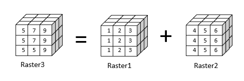
Map algebra is used as a general language in ArcGIS for processing and analyzing 2D rasters. Climate data has a third dimension (time), and some has an additional fourth dimension such as depth or height. The multidimensional Map Algebra capability makes analyzing climate data, or any scientific data, easier. The operators that you normally use for math, such as 3 = 1 + 2, can be used with 2D rasters, and these operators have also been enhanced to support multidimensional rasters.
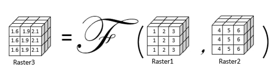
Dimension awareness of raster functions
Many raster functions have been developed to process 2D rasters and are dimensionally aware and support on-the-fly multidimensional raster processing (except for global functions). For example, the Remap raster function used in this study remaps for each 2D raster within the multidimensional raster, and the on-the-fly processed result can be saved as a multidimensional CRF.
Analyzing using ArcGIS Notebooks
Now I’ll start the process. I import ArcPy and the image analysis module (arcpy.ia), which includes the APIs that I will be using, and also check out the Image Analyst license, which is required by some functions.

Step 1: Create a raster object from the input CRF
I created a raster object from the CRF file. When you work with multidimensional rasters, make sure to set the second parameter, is_multidimensional, to True, otherwise you will end up with a 2D raster. You can see that the raster object created has two variables and the dimension array is 14,235, which includes the 39 years of daily temperature data.

Next, I filter the variables using the Subset function:

Step 2: Compute daily GDD
Daily GDD is calculated based on the maximum and minimum temperatures using this formula:
max ((max_temperature + min_temperature) / 2 – base_temperature, 0)
It is the average temperature above a base temperature and is 0 when the average temperature is below the base, since plants will not grow in such conditions. For grapes, I use a a base temperature of 10°C.
You can see that the multidimensional algebra makes the coding very simple, and I’m able to use operators on multidimensional rasters and compute the daily GDD over 39 years easily. Since the formula involves two rasters with different names, I must set an environment setting matchMultidimensionalVariable to False.

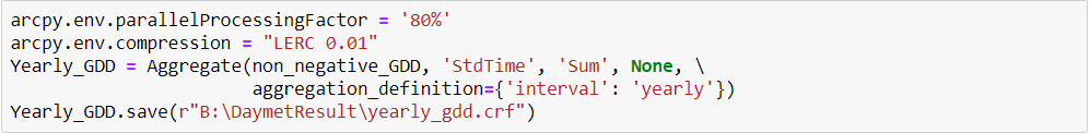
Step 3: Calculate yearly accumulated GDD
To calculate the total GDD of the growing season for each year, I use the Aggregate function and then save the process result as a CRF file. Since the dataset is large and the time series is long, I define the parallel processing factor and compression environment settings to speed up the process of data creation.
Step 4: Classification of wine growing suitability regions
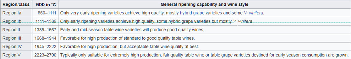
The Winkler index is a technique for classifying the climate of wine growing regions based on growing degree days. In the Winkler system, climate regions are classified as follows:
To apply the Winkler index to the analysis, I use the Remap raster function to remap the GDD ranges into six classes with values from 1 to 6:

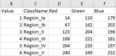
Now I have a multidimensional raster with values from 1 to 6 representing the six suitability regions. To associate the values with region names and the display color for each region, I create a CSV file containing a table with following records:
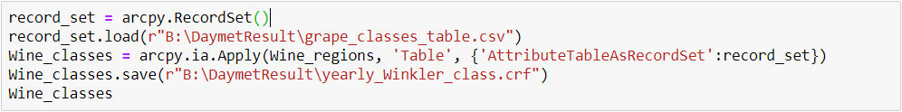
Next, I apply the table to the suitability region raster using a Raster Attribute Table function. Since there is not an explicit ArcPy function yet for the Raster Attribute Table raster function, I use Apply, an ArcPy function designed for processing using raster functions in ArcPy environment. In the code, ‘Table’ is the name of Raster Attribute Table function, and it takes a RecordSet as an argument. The result is a time series of wine suitability region classification from 1980 to 2018.
Step 5: Statistics of the suitability classes
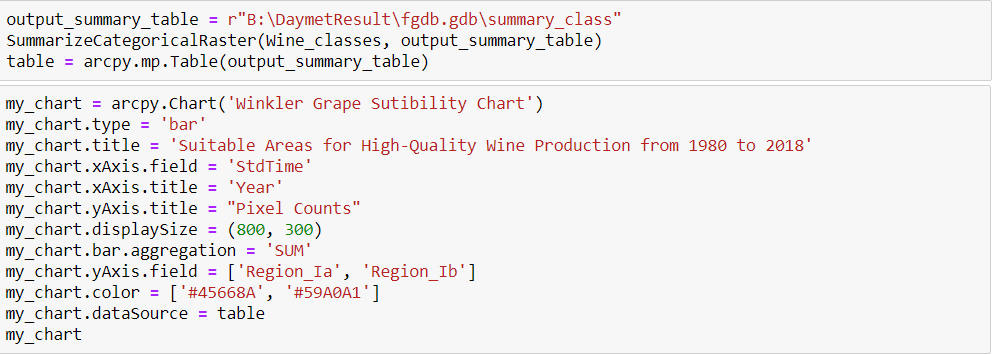
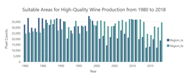
Last, to calculate the areas of the regions for each year, I use the Summarize Categorical Raster geoprocessing tool, which is newly released in ArcGIS Pro 2.7. The output table contains pixel counts for all region classes across all years. Then, I use an ArcPy chart class to display the trend of two classes.
The chart shows that Region_Ia, total areas (pixel counts) suitable for early ripened, high-quality grapes, are declining—which means that premium wines produced from these areas might be affected by the changing climate. The total pixel counts for Region_Ib and other classes do not show a big change over the years.
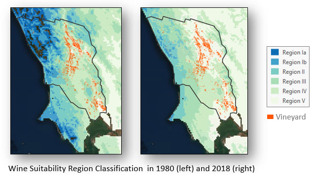
To find which areas are affected, I used the wine region classification time series generated previously, and compared changes in Sonoma, a county that produces the most and some of the best wines in California. You can see that areas suitable for high quality grapes and wines have shrunk, and the very few vineyards that were Region_Ia class in 1980 fall in Region III in 2018. Although there was no big change on the total pixel counts of Region_Ib, the areas shifted, which will affect the type and quality of grapes and wines produced in those areas
Summary
This is just one example of analyzing the climate’s impact on crops using multidimensional raster capabilities and ArcGIS Notebooks. You can apply similar workflows to other crops and many other types of scientific analyses across the areas of climate, weather, atmospheric, and ocean sciences. To learn more about multidimensional analysis and discover additional use cases, please watch our Directions Magazine webinar, Multidimensional Analysis: Trends, Prediction, and Change Detection

Nice!