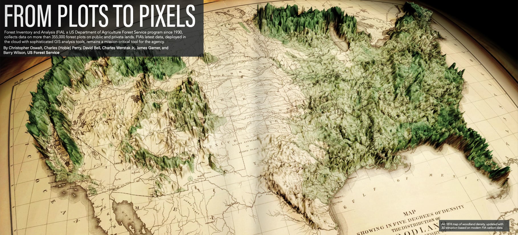
This is the map that introduces chapter 4 of GIS for Science Volume 3. It uses modern forest density data from the US Forest Service to give 3D elevation to an 1883 map of the same thing. Trippy. It was a fast and fun collaboration with Chris Oswalt and Hobie Perry of the Forest Service and publishing-pal Christian Harder.

Actually, I lied. The book’s graphic uses an 1873 map of forest density, but in this how-to I’ll use an 1883 version because I like it more.
…
0:00 Welcome to some mapping adventure! We’ll be making a graphic that uses modern forest density data to extrude a vintage map of forest density. So the 3D surface isn’t actual elevation, it’s forest density. You get it.
0:05 Finding this vintage map in the delectable David Rumsey Map Collection.
1:23 Completely optional step where I (off camera) Photoshop out the map scan’s edges so you only have the tattered map (relatedly, check out this fun resource if you are feeling bold).
1:41 Firing up ArcGIS Pro and starting with a Lambert Conformal Conic projection, to get a head-start on georeferencing.
2:48 Undoing the image enhancements Pro applies by default.
3:58 Let the georeferencing begin!
9:09 Quick conversion from 2D to 3D! So easy.
10:00 Adding a US Forest Service image service of “carbon density,” which is forest density.
10:45 Ah, it’s grayscale! We can trick ArcGIS Pro into thinking this is a digital elevation model! BWA HA HA HA HAAAAAA!
11:11 Cranking up the 3D scene’s vertical exaggeration to…12,000! You read that right.
11:57 Adding the trusty old “global background” layer from Living Atlas and giving it a picture fill of this wooden table top pattern.
12:57 Moving on over to a Layout. If you want to trick Pro into giving you more 3D detail, make your layout really big.
13:58 Hacking in a layout background color.
14:34 Adding a vignette. Because vignettes!
…
That’s it, friends! Thanks for hanging in there and getting all 3D-without-actual-elevation-but-with-some-other-data with me. So many happy trees.
Love, John


Article Discussion: