Using GeoAnalytics Server to detect delays in public transit

At the 2019 Esri Developers Summit plenary, we demoed how ArcGIS GeoAnalytics Server could be used to quickly identify important features in large collections of time-enabled data. For those interested in learning more about that demo, this blog post will go into more detail on how we pulled it off. Also be sure to check out a video of the analysis below!

Here are a few numbers that summarize the workflow:

• 3 million real-life bus locations
• 500 million simulated bus locations
• 100 cores of compute power across 3 servers
• 1000 GB of total RAM
• 5 minutes of total analysis time

In developing this demo, we wanted to use a dataset that would be relevant to GeoAnalytics users who are tracking moving assets like cars, buses, or people. Working with this type of data can be very difficult – both in terms of how long it takes to process and in knowing how to analyze or query the data to find answers. In this blog post I’ll explain how I used ArcGIS Enterprise 10.7 with GeoAnalytics Server to overcome these challenges by taking you through every step of the workflow, from gathering the data to finding patterns in the end result.

Gathering Data

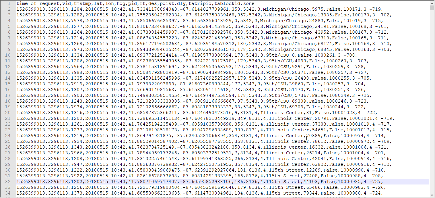
To create the input dataset for this analysis I used the Chicago Transit Authority Bus Tracker API to request and log the GPS coordinates and delay status of buses every three minutes for two weeks using a simple Python script. I wrote the data to an Amazon S3 bucket as a series of CSV files (check out a sample of the data below) and created a new file for every 100,000 records so that the files didn’t become too large and unruly. Because each file had the same schema, GeoAnalytics could read the entire collection of files as a single dataset, so I didn’t need to worry about combining the files into one massive file at any point (but I could have used just one file if I wanted to!). I also didn’t need to worry about moving the data anywhere to use it (phew!) because GeoAnalytics can read directly from data storage locations like S3.

Registering my data for analysis

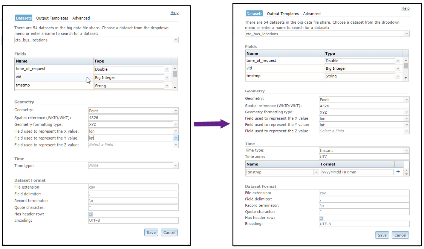
Next, I registered the S3 bucket containing my bus locations as a big data file share on my GeoAnalytics Server. This not only gave GeoAnalytics access to the data, but also defined how geometry and time are represented in my delimited files. When you register a big data files share, GeoAnalytics will read a small sample of each dataset and automatically discover the format of geometry and time fields. In the case that it’s unable to auto-discover these formats, they can be defined manually using Server Manager.

For example, when I registered my S3 bucket as a big data file share, “lat” and lon” were discovered as the geometry fields for my bus locations, but each feature in this dataset also had a timestamp that wasn’t discovered automatically. Because GeoAnalytics is so flexible when it comes to data registration, I was able to manually specify which fields contain time information and how that information is formatted. In this case, the “tmstmp” field contained string values in the format of “yyyyMMdd HH:mm”.

With both time and geometry fields registered correctly, I was ready to explore the data with GeoAnalytics.

To learn more, check out the web help for getting started with big data file shares and editing big data file share manifests in Manager.

Finding New Bus Delays with Detect Incidents

The Detect Incidents tool is unique to GeoAnalytics – it isn’t found anywhere else in the platform – and works specifically with track (time-series) data. Track data describes how things change over time, where each individual track represents a “thing”. Track data is often of interest because of a changing field, like a stationary air quality sensor logging measurements every hour (if that sounds cool, check out this video!).

In the case of my bus dataset, each bus location had a field called “dly” that indicated whether or not (True/False) a bus is delayed. I planned to analyze how this field changed over time to find out where buses became delayed.

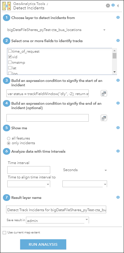
First, I needed to choose one or more fields in my dataset that defined which features belonged to the same tracks. I wanted each track to represent a unique route and bus, so I chose the “vid” and “rt” fields which represented the vehicle ID and route number of the buses.

Next, I needed to create an ArcGIS Arcade Expression that defined which features should be considered incidents and which should not:

Detect Incidents evaluated this expression for each feature in each track, labeling each one as an incident if the expression returned True, or a non-incident if the expression returned False.

The first line of my expression created an array representing a window of values in a track. Because I wanted to look at how the “dly” field changed between any two consecutive bus locations, I created an array containing the current value and previous value in time of the “dly” field.

In the second line of my expression, I returned True if the previous value in time equals “False” and the current value in time equals “True”. This means that the incidents in my result represented approximate locations where buses became delayed, hopefully revealing common causes of delay when we looked closer. To learn more about using Arcade expressions with Detect Incidents, check out this web help.

I used the Map Viewer in ArcGIS Enterprise to do this analysis. Map Viewer is a browser-based interface for performing analysis – one of many ways to access GeoAnalytics tools. After I finished filling out all of the required parameters, the tool looked like this:

The time it takes to complete this analysis depends on the number of cores and amount of RAM available on your GeoAnalytics Server site. I used 3 r5.12xlarge Amazon EC2 instances for my GeoAnalytics site and had adjusted my GeoAnalytics Server settings so that each job would utilize 100 cores and about 1000 GB of RAM total. I also had 3 r5.4xlarge EC2 instances running as spatiotemporal big data store machines and planned to write my result there (the spatiotemporal big data store is a type of ArcGIS Data Store). With this configuration, the analysis took about 30 seconds on 3 million points!

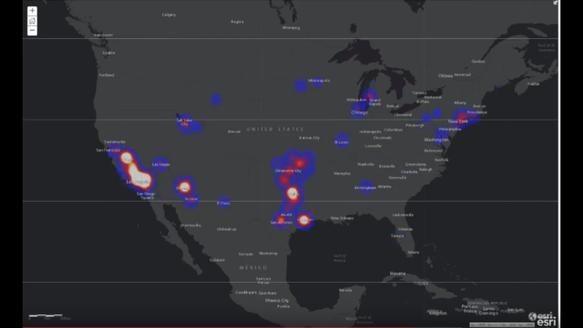
To visualize the result, I chose to symbolize on location only and selected the “Heat Map” option (not to be confused with hot spots!):

To test how much my GeoAnalytics Server could really handle, I duplicated the 3 million bus locations about 170 times, assigning new vehicle ID numbers to each duplicated set so that new tracks would be created. Running the same analysis on this dataset of more than 500 million records took only 4 minutes and 15 seconds!

That being said, you may not need a GeoAnalytics Server site with this much compute power to process your data in a reasonable amount of time. We require a minimum of 4 cores and 16 GB of RAM (though 32GB of RAM is recommended), and you can choose to scale this out only if needed.

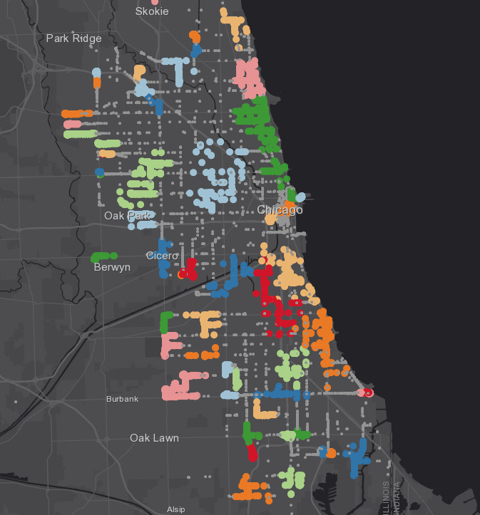
Finding Clusters of Delay Points with HDBSCAN

Visualizing my incidents provided a qualitative idea of where and when buses became delayed, but what if I wanted a more statistically significant assessment of the result? One way of doing that is with the Find Point Clusters tool, which gives you access to two density-based clustering algorithms, DBSCAN and HDBSCAN. These algorithms find clusters of points in surrounding noise, or in this use case, clusters of bus delays that could help pin point causes of delays.

I didn’t just choose to use HDBSCAN because I’m a fan of the letter H – the algorithm finds clusters with a variety of densities, whereas DBSCAN tends to find clusters of a similar densities. HDBSCAN also calculates a probability value for each cluster assignment, so I could evaluate the significance of my result. Besides choosing the algorithm, I just needed to provide one more parameter – the minimum number of bus delays that could seed a cluster – and I could run the tool. To learn more, check out this great ArcGIS Pro help topic on how density-based clustering works.

As mentioned in the DevSummit demo, the result reveals that many buses become delayed while passing through congested areas like mall parking lots and tourist attractions – though I don’t mean to throw those places under the bus!

With only two tools I was able to boil down 3 million points into a few dozen specific locations of interest. More importantly, the same analysis could be scaled out to 500+ million records with only 2-3 more minutes of analysis time!

This combination of easy-to-use spatiotemporal analytics and scalable compute is what makes GeoAnalytics so powerful, and this workflow is just the tip of the iceberg in terms of what can be done with these tools and others. If you are struggling to find answers in your large time-enabled datasets, you don’t want to miss the bus on this one!

Thanks for reading, and if you have any questions that I didn’t answer, or any questions on GeoAnalytics Server, feel free to email GeoAnalytics@esri.com.