Clean up your Landsat imagery: removing cloud and cloud shadow

The Landsat image archive is a great source for time series image analysis and change detection. Using Esri’s multidimensional raster analysis tools, you can explore time series image data to find out when, what, and where changes have happened.  But before you can analyze change, you need to get your image data ready for processing.

As you can imagine, the presence of clouds and shadow in a Landsat scene will affect the results of change analysis. The good news is that Landsat Collection Level 2 data, and Landsat Analysis Ready Data (ARD) for the U.S., comes pre-processed as surface reflectance and includes a Quality Assurance (QA) band containing information on cloud and shadow.  In this blog, we’ll show you how the QA band can be used for removing cloud and shadow from a single Landsat scene, or for a stack of Landsat scenes stored in a multidimensional raster dataset. This workflow can be done in ArcGIS Pro 2.7.

Note – if you don’t have Landsat Level-2 data or ARD data, and you just want to get rid of a few errant clouds on one image, check out this blog!

Clean up a single Landsat image

The example below uses Landsat 5 ARD data, but the same workflow can be used for Landsat 7 and Landsat 8 imagery.

When you browse to a Landsat 5 Collection 2 raster product (the one with the .xml extension) in the Catalog pane in ArcGIS Pro, there are two products listed: Surface Reflectance and the QA band.

The Surface Reflectance product is a multispectral image with 7 bands, while the QA product contains a single band with values describing the quality of the Surface Reflectance product. Using the Landsat ARD Format Control Book, we can see the list of QA codes and their meanings. Pixel values 66 and 68 correspond to land and water, while all other values are cloud and shadow with various levels of confidence.

To remove cloud and shadow from the Surface Reflectance product, we will use all the data covered by QA pixels with values 66 and 68, and set everything else to NoData.

Step 1: First, open the Remap raster function from the Raster Function pane, and set the input raster to the QA product. Specify pixel values 66 and 68 as valid, and set all other values to NoData.

Step 2: Next, use the Clip raster function on the Surface Reflectance product, where the clipping raster is the remapped QA product generated from step 1 above. This will cut out all the remapped NoData values from the Surface Reflectance image.

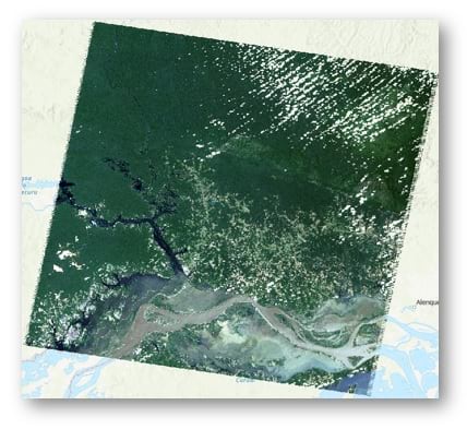
The output is a masked image, where areas of cloud and shadow appear as NoData. If you compare this image to another image for change analysis, areas of NoData will not generate incorrect change values from clouds or shadows.

You can use the same workflow to remove cloud and shadow pixels from Landsat 7 or Landsat 8 scenes; the only difference is that Landsat 8’s QA pixel values are coded differently from Landsat 5 and Landsat 7 QA products. You can use the Identify tool in ArcGIS Pro to click around on the Landsat 7 and Landsat 8 QA products to see which pixel values correspond to land and water vs. cloud and cloud shadow. 

Clean up a collection of Landsat images

Now you might be wondering: how do I apply a QA mask for a collection of images? For this workflow, you will apply the same two functions to a mosaic dataset when you are adding the data. Again, this example uses Landsat 5 ARD as an example.

Step 1: Create a new mosaic dataset using Create Mosaic Dataset geoprocessing tool. You can use all the defaults.

Step 2: Add the Surface Reflectance data using the Add Rasters to Mosaic Dataset geoprocessing tool.

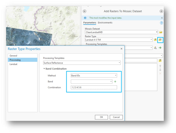
1. For Raster Type, choose Landsat 4-5 TM. Click the Raster Type property button to open the Raster Type Properties window.
2. In the Processing section, select Surface Reflectance for Processing Templates. For Band Combination, set the Method to Band IDs. I like to use band IDs because if I need to add Landsat 8 data, I can match the bands with 2 3 4 5 6 7 since in Landsat 8, the second band is the blue band. In this case, add bands 1-6. 

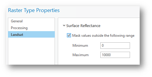
Both Landsat ARD and Landsat Collection 1 Level 2 Surface Reflectance products have pixel ranges classified as “all range” and “valid range.” We will include only pixels within valid range because negative pixel values outside the valid range will cause band index function to produce wrong result.

3. In the Landsat section of the Raster Type Properties window, check the box to Mask values outside the following range, and enter 0 and 10000 as the minimum and maximum, respectively.

4. Click OK to close the Raster Type Properties. In the Add Rasters to Mosaic Dataset tool, browse to the location of the folder of images as the input rasters.
5. It’s recommended that you check the box to Estimate Mosaic Dataset Statistics under the Mosaic Post-Processing section, as this will calculate the statistics for a better display.
6.  Run the tool.

Step 3: Add QA data to the mosaic dataset using the Add Rasters to Mosaic Dataset tool again.

1. Open the Add Rasters to Mosaic Dataset tool again. This time, after selecting the Landsat 5 raster type, set the processing template to QA. 
2. Click the Edit button next to the Processing Template parameter to define a custom template that will mask out pixels of cloud and shadow.
3. In the function editor, delete the Stretch function, and drag the Remap raster function from the raster function pane into the function editor. Connect the Dataset to the Remap function, then double-click on the function to open the Remap properties. Use the same settings we used for the single image above.

Click Save and close the function template editor

4. Again, browse to the folder containing your images as the input data. This time, do not check the box to Estimate Mosaic Statistics. We do not compute statistics anymore as we do not want to blend the statistics of the QA mask with the surface reflectance values.
5. Run the tool. When it’s finished, the dataset has two variables listed in the Tag field: SR and QA.

Step 4: Add the Clip raster function as a processing template to the mosaic dataset.

1. In the Catalog pane, right-click on the mosaic dataset and select Manage Processing Templates.
2. In the Manage Processing Templates pane, click the burger button in the top-right corner and select Create New Template. 

3. In the Raster Function Template editor, add the Clip raster function. Double-click on the function to open the Clip Properties window and click on the Variables tab. For the Raster parameter, set the Name to SR. For the ClippingRaster parameter, set the name to QA. This is important – the names of the input rasters much match the variable names we just added in the mosaic dataset. Click OK to close the Clip Properties.

4. Click the Edit Properties button. In the Edit Properties window, provide a name and description. Set the Type to Item Group, then type “groupname” as the Group Field Name and type “Tag” as the Tag Field Name. Uncheck the box to Match Variables.

5. Click OK and save the processing template.
6. In the Manage Processing Templates pane, click the star button in the upper right corner of the new processing template box to set it as the default template.

Step 5 (Optional): Now that your data is cleaned up, you can use it in multidimensional analysis tools! You’ll need to add the multidimensional metadata to the dataset.  Note that you only need to do this if you want to use multidimensional tools specifically.

And then use the Copy Raster tool to convert your multidimensional mosaic dataset to a multidimensional Cloud Raster Format (CRF) file. Below is a multidimensional CRF with cleaned Landsat scenes.

You now have a single Landsat scene,  a mosaic dataset, or a multidimensional CRF full of Landsat scenes where clouds and shadow have been replaced with NoData values! You can confidently use this imagery for change detection analysis without worrying about erroneous pixels or temporary changes from clouds.

If you want to know more about creating multidimensional raster data, check out this other blog.

For an example of performing change detection with a clean stack of Landsat images, watch this video on using LandTrendr, or check out the Continuous Change Detection and Classification example from the 2020 UC Plenary!

About the authors

Hong Xu

Hong is a Principal Software Product Engineer on Esri's raster team, where she has been working since 1999. She has played key roles in the development and leadership of various software products related to imagery and data science throughout her tenure. Currently, her areas of focus include time-series image analysis, multidimensional raster, and altimetry data.

Connect:

Julia Lenhardt

Julia is a product engineer on the Raster team. She has been with Esri since 2014 and has a background in remote sensing and GIS for environmental research. In addition to image analysis, she has a passion for music, running, good food and animal welfare.